Weekly commentary: MAT335 - Chaos, Fractals and Dynamics

14 January - Fractals

See the fractals page for some examples of fractals.

We have seen some bizarre geometric objects this week: the Cantor set (a set of uncountably many points whose length is zero), the Sierpinski triangle (an infinitely long curve outlining infinitely many triangles within triangles), the Menger sponge (an object with infinite surface area but zero volume; see page 108 in text), the Koch curve (a continuous curve that has no tangent line anywhere!), and the Peano space-filling curve (a curve that goes through every point in the unit square; see section 2.5 in text). All these objects were invented around 100 to 150 years ago by mathematicians to show how unimaginably complex geometric objects can be. These examples were motivation for mathematicians to re-examine the logical foundations of the subject, and spurred on the development of 'modern' analysis. Here's the quote by Freman Dyson as reproduced by Mandelbrot (page 3 in Mandelbrot's book): " Fractal is a word invented by Mandelbrot to bring together under one heading a large class of objects that have played an historical role in the development of pure mathematics. A great revolution of ideas separates the classical mathematics of the 19th-century from the modern mathematics of the 20th. Classical mathematics had its roots in the regular geometric structures of Euclid and the continuously evolving dynamics of Newton. Modern mathematics began with Cantor's set theory and Peano's space-filling curve. Historically, the revolution was forced by the discovery of mathematical structures that did not fit the patterns of Euclid and Newton. These new structures were regarded as 'pathological', as a 'gallery of monsters', kin to the cubist painting and atonal music that were upsetting established standards of taste in the arts at about the same time. The mathematicians who created the monsters regarded them as important in showing that the world of pure mathematics contains a richness of possibilities going far beyond the simple structures that they saw in Nature. Twentieth-century mathematics flowered in the belief that it had transcended completely the limitations imposed by its natural origins.
Now, as Mandelbrot points out, Nature has played a joke on the mathematicians. The 19th-century mathematicians may have been lacking in imagination, but Nature was not. The same pathological structures that the mathematicians invented to break loose from 19th-century naturalism turn out to be inherent in familiar objects all around us. (That is, Nature is full of these fractal-like objects.)

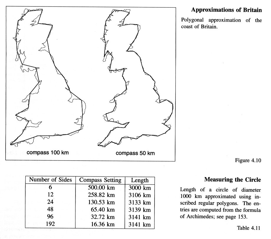
Measuring the length of curves.
( Larger view.) Given a ruler of a certain length (denoted by s in the text), we measure the length of a curve by placing the rulers end-to-end along the curve and adding up the number of lengths of the ruler needed to go from one end of the curve to the other (the length obtained in this manner is denoted by u in the text). 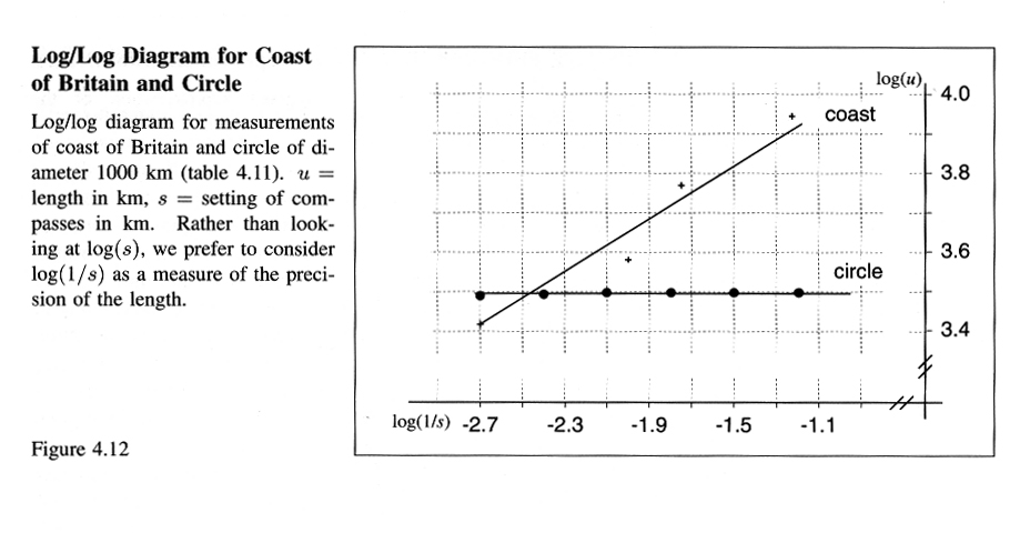This is an approximation to the length of the curve, but we showed in class that for regular curves, as the length s of the ruler tends to zero, the approximation converges to a finite number (which is the length of the curve). This should be familiar to you from your calculus class. And when you plot log(u) vs log(1/s) (or log(s) ) you obtain (nearly) a horizontal line (see Fig. 4.12 on page 194 in text). ( Larger view.)

The situation is different though for fractals and fractal-like curves. For example, for the Koch curve we find that the length of the curve increases without bound as the length of the ruler tends to zero! This means that as we look at the Koch curve more and more closely, we see more and more wiggles which makes the curve seem longer and longer (for regular curves, if you look at them closely enough they look like straight lines). Plotting log(u) vs log(1/s) for the Koch curve, we find that the line is not horizontal, but has a slope of d = log(4/3)/log(3) = .262 (see page 201 text). So, log(u) = b + d*log(1/s) (see equation (4.1) on page 194 of text). Taking the exponential of this equation we obtain that u = c* (1/s)^d, where c=exp(b). So you see that if the exponent d is greater than zero, then the length u tends to infinity as s tends to zero. And for larger d, u tends to infinity faster as s tends to zero. So those curves that have a larger exponent d must be more complicated than those curves with smaller exponents (the simplist curves are those with exponent zero; the regular curves). We will see that the exponent d is almost the same as the fractal dimension. So you see, the exponent d and the fractal dimension measure a qualitative feature of the curves; their complexity. (In homework question #7 you will estimate the exponent d for two curves; the coast of Britain and the coast of Spain. By eye, the Spanish coast looks more regular than the British coast so we expect that the exponent for the British coastline to be greater than the exponent for the Spanish coastline.)

• Section 2.5 (at least pages 94-98) of the text. This discusses Peano's space-filling curve.
• Section 2.6 ('Fractals and the Problem of Dimension')of the text.
• Section 3.1 ('Similarity and Scaling') of the text.
• Section 3.2 ('Geometric Series and the Koch Curve') of the text.
• Chapter 3 ('Dimension, Symmetry, Divergence') of Mandelbrot's book. This book is on reserve at Gerstein.
• Chapter 5 ('How Long is the Coast of Britain?') of Mandelbrot.
• Chapter 6 ('Snowflakes and Other Koch Curves') of Mandelbrot.
• Chapter 7 ('Harnessing the Peano Monster Curves') of Mandelbrot.
• Sections 14.2-14.4 and 14.6 ('Fractals') of Devaney's book. This book is on reserve at Gerstein.

Pascal's Triangle
Some remarkable, self-similar, patterns reminiscent of Sierpinski's triangle can be generated using Pascal's Triangle (see section 2.3 in the text). Pascal's Triangle is an array of numbers in the shape of a triangle. The top number is 1, and the row below that has 1,1 as entries. The third row of three numbers are generated by adding the two numbers above the number in the third row. This rule is used to generate the entire triangle (which continues indefinitely). Also, the nth row of Pascal's Triangle are the coefficients of the polynomial (1+x)^n. Now, if you colour the even numbers appearing in the triangle white, and the odd numbers black, a pattern similar to Sierpinski's Triangle emerges, and the pattern looks more and more like the Sierpinski Triangle as the size of Pascal's Triangle increases (see Figure 2.26 in the text). Instead of colouring even/odd numbers, which we can also describe as either being divisible by 2 or not, we can also colour those numbers appearing in the triangle according to whether they are divisible by 3 (white) or not (black), or whether they are divisible by 5 (white) or not (black), etc. What results are some very nice geometric patterns (see Figure 2.27 in the text). These patterns are the result of the number theoretic properties of the numbers occuring in Pascal's Triangle; this is discussed in section 8.1 of the text.