Overview of Begging Model PDF version
January, 2002
The begging model code includes a main program and five different groups of subroutines. Subroutines initialise the model (e.g., Init FileLoad), calculate statistics (e.g., Stats Main), report results (e.g., Report Graph) and implement the genetic algorithm (e.g., SexCrossover). One subroutine runs the nesting simulation (ModelFitness). This text focuses on the genetic algorithm and the nesting simulation.<
Italics identify model variables and parameters; underlined italics identify subroutines.
Data structures and parameters used by the genetic algorithm
The genetic algorithm manipulates four arrays that describe the "genotype" and "phenotype" of "parents" and "offspring" in a "population". Parent genotypes reside in oldchrom(ga.npop, ga.lchrom) and parent phenotypes reside in xParent(ga.npop, ga.nvar). Similarly, offspring genotypes reside in chrom(ga.npop, ga.lchrom) and offspring phenotypes reside in xchild(ga.npop, ga.nvar). Genotypes are single chromosomes (vectors of Boolean variables) of specified length (ga.lchrom) that are divided into a number of segments (ga.nvar), of equal, specified length (ga.lvar). The genetic algorithm decodes each chromosome segment into a base ten variable between zero and one. The phenotype is a list of variables from one decoded chromosome (the number of variables = ga.nvar). Population size is user specified.
User-specified parameters (read or calculated from the "chrom.dat" file) control the genetic algorithm (Table 1).
Table 1. Parameters used by the genetic algorithm.
|
Model Parameter |
Description |
Example Values |
|
ga.npop< |
the population size |
80 |
|
ga.nvar< |
the number of variables describing the phenotype |
5 |
|
ga.lvar< |
the number of alleles (Boolean variables) in each segment |
5 |
|
ga.lchrom< |
chromosome length (= ga.nvar x ga.lvar) |
5x5=25 |
|
ga.MaxDecode< |
the largest value a phenotype variable can take (= 2^ga.lvar — 1) |
2^5 — 1 = 31 |
|
ga.maxgen< |
the number of generations to model |
500 |
|
ga.pCross< |
the probability of crossover |
1 |
|
ga.pMutate< |
the probability of mutation |
0.02 |
|
ga.related< |
percentage relatedness of siblings |
50 |
Initialisation subroutines
The main program begins by calling InitMain. InitMain calls several other initialisation routines. InitFileLoad loads parameters used by the genetic algorithm from the "chrom.dat" file and parameters used in the nesting simulation from "enviro.dat". Files must be located in the same directory as the model. InitArrays creates arrays to hold variables. InitPop randomly assigns bits (true or false) to offspring chromosomes and decodes chromosomes into expressed strategies (by calling SexDecode; details below). It returns an array of offspring chromosomes (chrom(ga.npop, ga.lchrom); the first dimension holds the chick ID; the second dimension holds the alleles on the chromosome) and an array of offspring strategies (xchild(ga.npop, ga.nvar); the first dimension holds the offspring ID; the second dimension holds the decoded strategies)The main program then calls StatsMain. StatsMain calculates the mean and standard deviation of each offspring strategy variable for the current generation of offspring.
(italics identify model variables and parameters; underlined italics identify subroutines)Genetic algorithm subroutines
The main program then begins a repetitive loop that continues for the specified number of generations (gen goes from 1 to ga.Maxgen). It calls Growup, SexMain , StatsMain, ReportMain and ReportGraph within the loop.
Growup transfers values in the offspring arrays (chrom(), xChild()) to the parent arrays (oldchrom(), xParent()), signalling the passage of a generation. A generation counter (gen) is incremented immediately before Growup is called. Parents are now ready to produce offspring and enter the nesting simulation.
SexMain calls SexSelectParent, SexCrossover, SexDecode and SexFitness. SexMain has different sets of routines for scenarios where siblings are either 0, 50 or 100% related (choice specified in "chrom.dat"). We only discuss routines for 50% relatedness below.
SexSelectParent selects two parent genotypes randomly (with replacement) from the parent array (oldchrom()).
SexCrossover creates one offspring chromosome from two parents. Ga.pCross determines the probability of crossover occurring (usually ga.pCross = 1). The crossover position is determined randomly. If ga.pCross takes a value of less than one, then strategies from one parent may pass directly to an offspring. SexCrossover assigns values to the offspring chromosome from one parent up to the crossover point and from the other parent after the crossover point. Mutation may occur during assignment. SexCrossover calls SexMutation to cause mutation with a probability specified by ga.pMutate. SexCrossover runs twice to create two offspring chromosomes.
SexDecode translates the binary vector on the offspring chromosomes (chrom()) into base-ten variables (xchild()) that describe begging behaviour and provisioning behaviour (the phenotype).
SexFitness simply assigns more meaningful names to variables describing offspring behaviour. Y1a describes the Alpha nestling’s begging level at its minimum relative condition; Y2a describes begging level when in maximum condition. Similarly, the Beta nestling’s begging level is described by Y1b and Y2b. Linear interpolation calculates begging level at intermediate relative conditions. SexFitness also assigns a more meaningful name–pFeedNoisy–to the variable describing parental provisioning behaviour (the provisioning parent was selected randomly in SexMain ). Finally SexFitness calls ModelFitness–the nesting simulation–to assess the survival of the nestlings, given their strategies, parental strategies and environmental conditions.
Back in SexMain, offspring that survive the nesting simulation are added to the population of parents forming the next generation. SexMain continues to select parents, create offspring and assess their performance in the nesting simulation until the number of surviving offspring reach the desired population size (ga.npop).
Data structures and parameters used by the nesting simulation
The nesting simulation models Alpha (first born) and Beta (second born) nestlings. Variables and parameters include the letter "a" or "b" when they refer to the Alpha or Beta nestling respectively. The nesting simulation uses parameters passed from the genetic algorithm and parameters specified in the "enviro.dat" file (Table 2).
Table 2. Parameters used in the nesting simulation.
|
Model Parameter |
Description |
Example Values |
|
Y1a |
begging level of Alpha nestling at minimum relative condition |
0 — 1 |
|
Y2a |
begging level of Alpha nestling at maximum relative condition |
0 — 1 |
|
Y1b |
begging level of Beta nestling at minimum relative condition |
0 — 1 |
|
Y2b |
begging level of Beta nestling at maximum relative condition |
0 — 1 |
|
pFeedNoisy |
probability that parent feeds the noisiest nestling |
0 — 1 |
|
sim.Foodsupply |
amount of food brought by the parent each feeding |
near 2 |
|
sim.aMaxBegCost |
energetic cost of begging at the maximum level for the Alpha nestling |
0 = no cost |
|
sim.bMaxBegCost |
energetic cost of begging at the maximum level for the Beta nestling |
0 = no cost |
|
sim.aNeed |
multiplied by food to reduce or increase energy obtained from food (Alpha nestling) |
1 = no effect |
|
sim.bNeed |
multiplied by food to reduce or increase energy obtained from food (Beta nestling) |
1 = no effect |
|
sim.bhandicap |
used to increase risk of starvation |
0 = no effect |
|
sim.Predation |
the risk of predation at the maximum begging level of both chicks |
0 = no predation |
|
sim.ability |
changes the begging level of the A chick without increasing begging costs; a value greater than one increases begging level |
1 = no effect |
|
sim.starve |
starvation risk when in minimum condition |
0 = no risk 1 = full risk |
Nesting Simulation
The nesting simulation resides in the ModelFitness subroutine that is called from SexFitness within SexMain. It simulates changes in nestling condition, and ultimately nestling survival to fledging, in response to the begging behaviour of Alpha and Beta nestlings, the provisioning behaviour of the parent and environmental conditions.
Environmental parameters set food available (sim.Foodsupply), starvation risk (sim.starve) and predation risk (sim.Predation). Predation risk affects both nestlings.
Nestling state is described by relative condition. The model tracks the absolute condition of each nestling(Xa, Xb), but uses relative condition–deviation from a theoretical average condition (DeltaXa = Xa — Xmean, DeltaXb = Xb — Xmean)–to serve as the basis for calculations. Average condition (Xmean) increments by 0.5 each time step.
Nestlings enter a 100 time-step simulation that models starvation, begging, predation, feeding and changes in condition. Starvation and begging level are modelled first for each chick. Then, predation and feeding are modelled using both nestlings. Finally, changes in condition are modelled for each nestling.
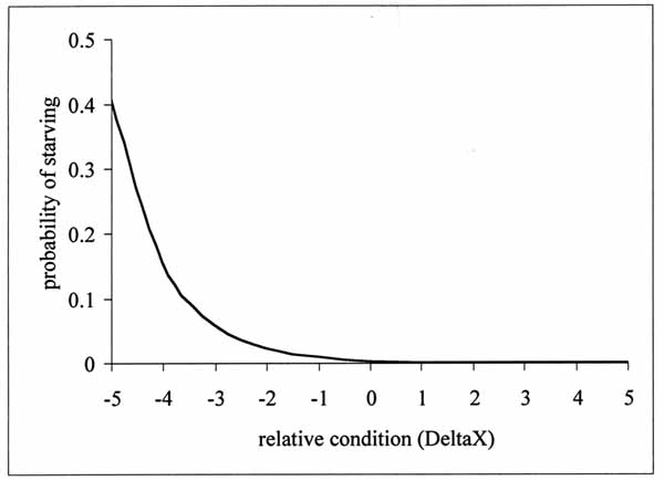
Starvation risk (Figure 1) depends on relative condition (DeltaXa, DeltaXb) and the starvation parameter (sim.starve). Changes in food received and other factors affect condition, which in turn affects starvation risk. Sim.starve changes starvation risk for a given condition. When sim.starve equals zero, starvation does not occur.
Figure 1. Probability of starvation (when sim.starve = 1) versus relative condition.
If a nestling survives the starvation routine, the model calculates its begging level (abeg, bbeg). Begging level depends on a nestling’s condition and begging strategy (Y1a, Y2a, Y1b, Y2b), describing begging levels at minimum and maximum condition (begging level changes linearly with condition). The genetic algorithm determines begging strategies. The begging level of the Alpha nestling can be further modified by the begging ability parameter (sim.ability). Usually this parameter is used to give the Alpha nestling a higher begging level at a given condition (e.g., assuming the Alpha nestling is older or larger) without increasing metabolic costs. The begging level of the Beta nestling is not modified.
Once the begging levels of both nestlings are determined, nestlings enter the predation and feeding routines. The probability of predation increases linearly with the combined begging level of the Alpha and Beta nestlings, relative to the maximum level that they can both beg. The predation parameter (sim.Predation) defines the predation risk at the maximum begging level. No predation occurs when sim.Predation equals zero.
At the beginning of the feeding routine, the parent chooses to feed either the quiet or the noisy nestling. The probability of feeding the noisy nestling is encoded on the parental chromosome. Then, when both nestlings are alive, the model determines which nestling is noisiest. Allocation of food depends on which nestling is noisiest and on parental choice. If only one nestling is alive, the model feeds it.
The model then updates the relative condition of each nestling. First it determines the proportion of the food that can be used (aFoodValue, bFoodValue) by a nestling, considering relative condition and long term need (sim.aNeed, sim.bNeed). FoodValue declines for chicks in above average relative condition (Figure 2). FoodValue changes in proportion to changes in long term need. Then, the model calculates the "metabolic" cost of begging. Begging cost increases in direct proportion to begging level. Finally, the relative condition of a nestling is calculated as energy gained (FoodLoad x aFoodValue) minus energy lost for body maintenance (a constant, Cm) and energy lost to begging (abegcost, bbegcost). After relative condition is calculated, the nesting simulation moves to the next time step and repeats the calculations described above.
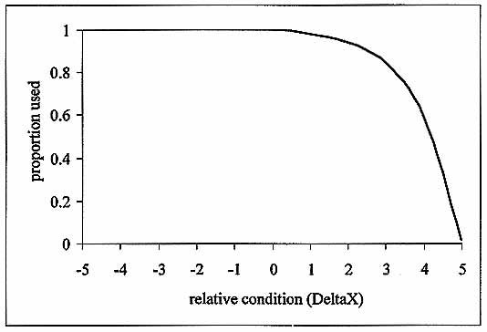
Figure 2. Proportion of food energy used versus relative condition when long term need equals 1.
Results files
The model produces three results files (in text format). "Detail.out" describes offspring phenotype, for each member of the population for selected generations. It lists the means and standard deviations for the population. "Plotvar.out" reports the averages and standard deviations of phenotype variables in the offspring population for selected generations. It reports the number of Alpha and Beta nestlings that die in each generation. At the end of the file, it reports the means and standard deviations of the phenotype averages and of the nestling deaths for the last 50 generations in the simulation. "DeltaX.out" reports the mean, maximum and minimum relative condition of the Alpha and Beta nestlings in the last generation of the nesting simulation. It also reports the last time period when the each nestling was alive (100 indicates the nestling survived the nesting period).
Parameter files
Tables 3 and 4 list parameter values that we have frequently used, for reference. The model uses one parameter file to control the genetic algorithm ("chrom.dat") and one to control the nesting simulation ("enviro.dat"). In "chrom.dat", setting num_var to 4 creates a parent that always feeds the noisy chick. Setting num_var to 5 allows parental feeding strategies to evolve. Mutation rates of 0.01 or 0.02 provide an "appropriate" amount of new variation. The genetic algorithm should be run for at least 200 — 500 generations to allow good strategies to emerge. Relatedness may be set to 0, 50, or 100, with 50 being appropriate for siblings (the model does not handle intermediate values). In "enviro.dat" we varied food supply, predation rate, the ability of the Alpha chick, the long-term need (bHandicap) of the Beta chick and the starvation risk.
Table 3. Parameters stored in "chrom.dat". Bold indicates default values
|
Parameter Name (in file) |
Typical Values |
||||||
|
pop_size |
80 |
||||||
|
num_var |
4 or 5 | ||||||
|
var_len |
5 |
||||||
|
num_gen |
|||||||
|
200 — 500 (must be > 50) |
|||||||
|
p_cross |
1 |
||||||
|
p_mutation |
0.01, 0.02 | ||||||
|
Related_(0,50,100) |
0, 50, 100 |
||||||
Table 4. Parameters stored in "enviro.dat". Bold indicates default values
| Parameter Name (in file) | Typical Values | ||||||
| Food | 2, 2.1, 2.2 | ||||||
| aMaxBegCost | 0 | ||||||
| bMaxBegCost | 0 | ||||||
| aNeed | 1 | ||||||
| bNeed | 1 | ||||||
| Predation | 0, 0.01 | ||||||
| aAbility | 1, 0.67, 1.5 | ||||||
| bHandicap | 0, 1 | ||||||
| starve | 0.25, 0.5, 1 | ||||||