Fraser Floods Research Group

Study Region

The Fraser Basin lowland region extends from Hope to the Strait of Georgia, British Columbia. This area comprises several municipalities that are at potential risk should an extreme flood event occur. Although a thorough examination of an extreme flood event on the Fraser River would ideally encompass the entire extent of the Fraser Basin lowland, in this case the study area was naturally limited to the extent of the high resolution LiDar Digital Elevation Model which extended from Hope to Abbotsford, B.C.

Geology of the Fraser River Basin

The Fraser Lowland and adjacent Georgia Depression are underlain by three distinct basements that make up the Vancouver region. To the north the granitic Coast Mountains; to the south-east the volcanic and sedimentary Cascade Mountain Range; and to the west the Vancouver Island Insular Belt, made up of volcanic and sedimentary rocks. The topographic lows that contain the Georgia Basin and the Fraser Lowland region correspond to the boundaries of the three basements. Sedimentary rocks of Upper Cretaceous and Tertiary age unconformably overlie these basements in the Vancouver region, while the Fraser Lowland region overlies roughly 2.5 km thick Tertiary sequence [Figure 1] made up of fluvial deposited conglomerates and sandstones (Clague 1998).

Pleistocene glaciation extensively impacted the Vancouver region. During the final advance of the Fraser Glaciation 15,000 years ago the Cordilleran Ice Sheet covered the Vancouver area under a piedmont lobe glacier roughly 2 km thick (Clague 1998). The ice sheet had retreated by 11,000 years ago leaving behind Quaternary sediments several hundred meters thick in the Fraser Lowlands [Figure 1]. After this retreat the Fraser River flowed into the Strait of Georgia which was positioned as far east as New Westminster (Eisbacher 1973). Between 10,000 and 8,000 years ago deposition of sands, silts and clays were deposited and the Fraser River Delta was formed (Eisbacher 1973).

Hydrological Regime of the Fraser River

The Fraser River is 1400 km long and originates in Fraser Pass, 2,015 meters above sea level and meanders north-west to Prince George where it turns southward. After passing through the Fraser Canyon the river turns westward near Hope and from there flows through the Fraser Lowlands and drains into the Strait of Georgia. Several major tributaries feed into the Fraser River including Stuart River, Harrison River, Thompson River, Chilcotin River, Nechako River and Quesnel River (Shrestha et al. 2012). The drainage basin area that encompasses the Fraser River and its several tributaries is 234,000 km, or roughly ¼ the size of British Columbia. This large basin area accounts for the Fraser River’s slow response time to meteorological events, as well as its ability to absorb normal occurrence events without resulting floods.

Typically, winter discharge on the Fraser River is low despite substantial precipitation from storm events in the region. The winter precipitation is predominantly accumulated and stored in the catchment as snow. The hydrologic regime of the Fraser River is in turn controlled by snow accumulation and associated snow melt processes (Shrestha et al. 2012), although the hydrologic response at different locations within the basin can vary from being rain controlled to snowmelt controlled to a hybrid of snowmelt-rain controlled. Although roughly 1.5% of the basin area remains glaciated, glacial melt and processes contribute little to the hydrologic regime of the Fraser River (Shrestha, et al. 2012). Overall, snowmelt comprises the largest source of water for the Fraser River. The hydrograph of the Fraser River [Figure 2] shows the annual discharge is approximately 112 km3 per year, with the annual peak flow occurring from May through August to coincide with the snowmelt leading to the spring freshet (Dashtard and La Croix 2015). In addition to the large water discharge load the Fraser River carries it also transports over 20 million tons of sediments annually, mostly as suspended sediments but also as coarse bedload (Eisbacher 1973). It is this sediment transport that has built the Fraser Delta and has created the rich agricultural Fraser Lowlands.

Contributing Climatic Influences

Many climatic factors influence the hydrologic regime, discharge levels and flood risk on the Fraser River. The climate in B.C. is strongly influenced by its proximity to the Pacific Ocean and several North-South oriented mountain chains. The atmospheric regime is dominated by prevailing Westerlies that carry in moist air parcels from the Pacific (Shrestha et al. 2012). Orographic lift results in heavy precipitation in the mountain ranges. The majority of frequent winter storm events experienced in the Fraser Basin originate in the North Pacific Ocean. Occasionally a cold dry Arctic air front will collide with the warmer Pacific air and result in substantial snowfall, even near sea level.

The region is also impacted by Pineapple Express (PE) storms that develop in the Pacific Sub-tropics. These storms occur between 1 and 4 times a year and cause extremely heavy precipitation. These subtropical storms are accurately referred to as ‘atmospheric rivers,’ several hundred kilometers wide and more than 2000 km long, these rivers are responsible for over 90% of global water vapor transport at rates that exceed 20 km3 per day. The rapid influx of this vapor into the Fraser River Basin results in extreme precipitation and is known to initiate precipitation induced natural hazards such as floods and landslides (Spry et al. 2014).

Mechanisms Responsible for Past Flood Events

Of the floods on record, two stand out due to their extent or human impacts: the flooding events of 1894 and that of 1948. The event of 1894 caused flooding from Harrison to Richmond, BC. The flooding began on May 25th, reaching a peak on June 10th. Although this flood’s extent was never mapped, an understanding of its record-breaking levels was recorded in New Westminster with 13 ft and 9.5 inches (4.2m) over the low water mark. Low lying areas such as Annacis Island were completely submerged (Szychter 2000). In response to this destruction, the Federal Government instituted a Farmer’s Relief fund as all crops were destroyed in low-lying areas.

The 1948 prevailing conditions were similar to the 1894 event with a hot May preceded by a winter with high snowfall, but flooding was not as extensive (Fraser Basin Council 2014). The discharge was measured to be 15,200 m3/s at its highest with heights of 7.6m at Mission (Vancouver Sun Library 2012). Vancouver, for the first time since railways had been built, was cut-off by land as railways were washed out. The federal government response was swift: the Army, Navy and Air Force were deployed to evacuate stranded citizens, reinforce diking infrastructure, and clear debris (New York Times 1948). In total, 16 000 individuals were evacuated, 10 were killed and 2300 homes were destroyed. The economic repercussions were a loss of $210 million in today’s dollars. The high number of individuals affected, and the high economic losses incurred were likely due to an increase in population since the 1894 event (Fraser Basin Council 2014).

Flooding Events

Several factors have contributed to historic flood events on the Fraser River. In order to generate an extreme magnitude event such as a “200-year flood” event, that is a magnitude event that is likely to occur once every 200 years on average, a near perfect confluence of these factors must occur. The primary mechanism responsible for past flooding events is a ‘rain on snow’ event (Clague and Turner 2003). This occurs when a winter of heavy precipitation that has resulted in substantial snowpack in the mountains is followed in the spring by a single heavy precipitation event. These events are known to increase hazard potential of floods and landslides. Historic floods on the Fraser River are associated with multiple PE events during the preceding winter, and concerningly several current studies have demonstrated that global warming will likely exacerbate PE events (Spry et al. 2014), in turn increasing the likelihood of flood events on the Fraser River. Rain on snow event are unique in that they create a catalyst by which multiple precipitation events that have been stored in the basin as snow and ice are simultaneously released from storage. This is possible due to the difference between the latent heat of fusion and the latent heat of vaporization. When water vapor condenses to liquid it releases 2260 kJ/kg of energy. The energy required to melt snow or ice is only 334 kJ/kg. Therefore, condensing water vapor is capable of melting nearly seven times the equivalent amount of snow and ice. This can result in the equivalent of multiple PE events along with several smaller winter storms all releasing into the Fraser River’s flow regime at once.

Flood Management and Preparedness

The 1948 flooding event spurred government action. From 1948-1968, the federal government entered an agreement with the provincial government to cover 75% of the costs for new infrastructure that could prevent flood damage in the event of another 1894-type flood. This agreement was modified in 1968 until 1995 in which the coverage was reduced to 50%. In total, 250 km of dikes, 84 km of bank protection and more than 100 alternative structures for flood management were constructed to protect the populated and farming areas of the Fraser Basin. In theory, approximately 55,000 hectares of floodplain would be saved by these measures if there was another flood like the 1894 event (Day 1999).

After the 1948 flood, estimates of flood inundation extent were made by the federal and provincial authorities to build the new diking systems to mitigate flood damage that would likely occur should another catastrophic event similar to that of 1894 happen. Since 1995, the onus for maintaining and building dikes largely falls on agreements between the provincial and municipal governments (Day 1999). In the 1980s, the province took an interest in extensively mapping flood risks throughout BC, but loss of funding led to the demise of continuing these efforts (Day 1999).

Today, flood management response is via Emergency Preparedness Canada (EPC), an initiative of the federal government to train and educate the public on disaster awareness as well as act as a parent organization to provincial emergency authorities (Day 1999).

The Fraser Basin Today

The lifting of development bans on at-risk areas in the Fraser Basin in the 1970’s has allowed for the increase of the population living in at-risk areas to what it is today an estimated 300 000 people (Fraser Basin Council 2014). With climate change affecting the basin, a flooding scare occurred in 1999 that reminded authorities of the need for better flood management. Given that communities in the Fraser Basin are home to two thirds of the population of BC and account for 80% of the provincial GDP, a disaster similar to the 1894 event would cause serious economic losses (Day 1999). According to the most recent findings, a Fraser River flood of such magnitude would cause at least $22.9 billion in losses (Fraser Basin Council 2016b).

Infrastructure and Mitigation

The current Canadian flood management system is implemented from hazard based management models. This means that infrastructure and flood mitigation along the Fraser River has been based off the likelihood that a 200-year flood similar to the 1948 event will occur again (Jakob, 2011). Frequency and severity of flooding in most of the world has increased over the past decade. Switching to a risk based system of flood management could help drastically reduce the impacts that a 200-year flood would inflict upon the lower mainland. A risk-based system would calculate flood vulnerability based on statistical variables and proper planning could be applied to mitigate impacts.

Macromodeler

Data

We acquired submeter LiDar data from the Fraser Valley Regional District. The data was provided in the form of several .las files that we have converted to a Digital Elevation Model or DEM for short. The DEM was then converted to a .rst file using Terrset. We aggregated the data by a factor of four. Each of the inputs for the CA were created by using the DEM in ArcMap. We were able to identify the dikes and create a shapefile in order to subtract the height from the CA so the buffer would not ignore the dikes. An initial polygon was created in ArcMap to serve as a starting point for the flood. High quality data is required for this project because having a high quality DEM is crucial for the accurate modelling and analysis of floods (Guidolin 2016; Jones 2004).

Methods

Cellular automata is a method of performing geographic analysis in both space and time (Berto, 2017). In recent years, GIScientists have developed increasingly effective models in order to simulate floods, cellular automata is one of many (Guidolin 2016). A cellular automaton at its core is a simple matrix of cells that represent a geographic space (Berto 2017). Because a cellular automaton is a matrix of cells, cellular automata is a form of raster based analysis. The individual size of pixels within the matrix is important depending on the phenomenon you are representing. In this case, we wanted a very fine resolution to accurately model the dikes as well as to create an output that is as accurate as possible. We thought this was important because of the scale of potential damage. Each cell in the matrix has a state. A cellular automaton can have several states, but for the purpose of this project our model only requires two, flooded and not flooded.

Macro Modeler

We created our model using Terrset’s Macro Modeler. You can view our macro modeler above. Our modeler is composed of an initial starting point map which is then buffered, this process will be described in the next section. This image is then overlain by multiplication with our aggregate image, that has been through a fuzzy. This produces a suitability map that decides which cells have potential to change. This image is then processed by toprank, which prevents a specified percent of the highest elevated cells from transitioning. We then cover the initial flood position with the toprank output. This is the new map that shows which cells have flooded. The output of the first iteration becomes the initial flooding point for the second iteration. The first iteration output is also overlain by addition with the aggregate image. The aggregate image is also updated every iteration. All of these steps are repeated every iteration, for 25 iterations.

Buffer and Toprank

We ended up having to use a buffer because the original filter stopped working after several iterations. The key difference being that the buffer is circular, unlike filter which was square. The shape of the buffer or filter will affect the shape of the spread. The buffer was set to a size of 400 units, meaning about 1600m. The buffer size was chosen because it required fewer iterations to produce the same outcome as a smaller buffer size. This saved a lot of hard drive space.

Toprank was used to select a portion of cells that would not flood each iteration. We selected a value of 90%. Meaning that 10% of the highest elevation cells did not transition. We calibrated toprank with several different values including 99, 95, 75 and 50 percent. 90% had a more realistic output than 95 or 99 percent tests while the 75 and 50 percent iterations produced errors.

Suitability Map

Our Cellular Automata uses a suitability map to determine whether or not a cell is suitable to transition from non-flooded to flooded. The suitability map is produced by multiplying the buffer output with the fuzzy aggregate image. Our weighting system for our suitability map is simple because elevation is the only factor, and therefore rated as 100%. The transition rules affecting floods are easily weighed because elevation is the primary factor. This is a key assumption that we are making in our model. Our suitability map is a digital elevation model of the lower Fraser Valley. Although floods are difficult to model, due to the inability to properly encompass the complexity of floods; useful information can be gathered from relatively simple analysis (Guidolin 2016). Which is why we only need one factor in order to conduct our analysis. The use of only one factor is supported by our theoretical background research.

Iterations

Initial Flood Starting Point

A cellular automaton isn’t, as previously stated, solely a spatial modelling technique; it also captures phenomena over time. Cellular Automata incorporates the temporal aspect of geographic events by producing a specified number of iterations. An iteration is a time step that uses the previous iterations’ output as the new input. The number of iterations should be representational of the dynamics of the specific flood. Our iterations do not represent a specific quantity of time. Unfortunately, the exact rate of the rising flood waters was not recorded in 1894 or 1948. Because of this we selected a simulation length of 25 iterations because it was best at representing the possible extent of the flood. With more data we could alter the amount of water added each iteration while also limiting the number of iterations to the volume of water that would be involved during a flooding event. Floods can only spread as far as the volume of water allows, even if there is more low ground.

Key Assumptions

Incorrectly assuming the cause of a future flood could have devastating implications on management strategies. We are assuming that the flood will be generated by severe rain on snow events as indicated by historical events and studies (Szychter 2000; Fraser Basin Council 2014). For the purposes of this model we also have to assume there is no climate change and that flood dynamics remain the same in the future, it is unlikely that this will hold true. Most flood modelling techniques do not account for lateral water transfer (Chen 2009). Lateral water transfer is difficult to measure because the transfer is unobservable without precise measuring equipment (Chen 2009). Lateral water transfer does not severely impact modelling the geographic extent of floods (Cai 2008; Chen 2009; Guidolin 2016). In order to simplify each iteration we have assumed that the flood waters rise at a constant rate. Unfortunately, no hydraulic data exists for either the 1948 or 1894 floods, this data would have allowed us to fine tune the model. Finally, we ultimately had to select an initial flood point for the cellular automaton. The simulation requires a point of origin; we have selected the whole Fraser River as the starting point in order to represent the effect of a flood with a slow build up.

Results

The result of our CA did not meet our original expectations; this is due to multiple reasons including the limitations of time, data availability, processing power and data storage. The original goal was to create a hydrologically accurate output. This quickly became impossible due to the lack of hydrological data. With the challenges we faced in mind, we would require at least another semester to work out all the kinks in the project. Our original goal for this project was very optimistic.

The results of the CA are very easy to interpret. You can view the extent of the flooding in the GIF. As expected the flood spreads further every iteration. The spread is very circular in shape; this is because of the buffer. The buffer size would have to be decreased in order to fix this, but that would drastically increase simulation time and the amount of data.

Errors were created in many ways. The edge of a raster causes error propagation within CA’s due to how they affect the shape of the buffer. Extreme values within a few swathes of the LiDar data has caused flooding in areas that shouldn’t be flooded when compared with a map. The incorrect LiDar values also caused stretching in the aggregate and in the CA. One issue with the CA that is immediately identifiable is the fact that the flooding passes in between gaps on the outer edge of our data. This means that our map is forecasting flooding where there shouldn’t be any, but this is not the fault of the model.

We would like to thank Fraser Valley Regional District for providing us with the valuable LiDAR data of the Fraser Valley. Further we would like to thank our project liaison John Clague for his valued input in defining the scope of the study and his continued advice. We would also like to thank David Swanlund for providing technical support and Nadine Schuurman for guidance.

BBC. KS3 Bitesize geography. Retrieved from http://www.bbc.co.uk/bitesize/ks3/geography/physical_processes/rivers_flooding/revision/7/.

Berto, F. 2017. Cellular Automata. Stanford Encyclopedia of Philosophy. https://plato.stanford.edu/entries/cellular-automata/

Breckenridge, J. 1895, December 26. A WILD NIGHT ON THE FRASER.: Afloat in a Flood on a Ferry-Raft.--A Work of Rescue. The Youth’s Companion (1827-1929); Boston,: 665.

Burakov, D.A., and Ivanova, O.I. 2010. Analysis of formation and forecast of spring snowmelt flood runoff in forest and forest-steppe basins of Siberian rivers. Russian Meteorology and Hydrology, 35: 421–431. doi:10.3103/S1068373910060099.

Burrel, B.C., Davar, K., Hughes, R. 2007. A Review of Flood Management Considering the Impacts of Climate Change, Water International, 32:3, 342-359, DOI:10.1080/02508060708692215

Cai, X., Li, Y., Guo, X., Wu, W. 2014. Mathematical model for flood routing based on cellular automaton. Water and Science Engineering. Vol. 7(2). pp.133-142/. doi:10.3882/j.issn.1674-2370.2014.02.002.

CGEN. 1995. Vancouver-Fraser Floods. Available from http://www.cgenarchive.org/vancouver-fraserfloods.html [accessed 25 February 2018].

Chen, J., Hill, A., Urbano, L. 2009. A GIS based model for urban flood inundation. Journal of Hydrology. Vol 373. Pp.184-192.

Chow, V. T. 1962. Hydrologic determination of waterway areas for the design of drainage structures in small drainage basins, experimental station bull. Illinois: University of Illinois, Engrg.

Clague, J., Luternauer, J., Mosher, D. 1998. Geology and Natural Hazards of the Fraser River Delta, British Columbia. Geological Survey of Canada. Bulletin 525.

Clague, J., Turner, B. 2003. Vancouver, city on the edge: living with a dynamic geological landscape. Pp.67-77

Dashtard, S.E., La Croix, A.D. 2015. Sedimentological trends across the tidal–fluvial transition, Fraser River, Canada: A review and some broader implications

Day, J.C. 1999. Planning for floods in the lower Fraser basin, British Columbia: toward an integrated approach. Environments; Waterloo, 27: 49.

Eisbacher, G. 1973. Vancouver Geology: A Short Guide prepared for the Geological Association of Canada. Pp. 47-49

Fraser Basin Council. 2014. Flood and the Fraser. Available from https://www.fraserbasin.bc.ca/water_flood_fraser.html [accessed 15 February 2018].

Fraser Basin Council. 2016a, May. Lower Mainland Flood Management Strategy. Available from https://www.fraserbasin.bc.ca/water_flood.html [accessed 23 February 2018].

Fraser Basin Council. 2016b. Lower Mainland Flood Strategy: Phase 1 Summary Report. Fraser Basin Council. Available from https://www.fraserbasin.bc.ca/_Library/Water_Flood_Strategy/FBC_LMFMS_Phase_1_Report_Web_May_2016.pdf.

Guidolin, M., et al. 2016. A weighted cellular automata 2D inundation model for rapid flood analysis. Environmental Modelling and Software. Vol 84. Pp.378-394.

Jain, S.K., Mani, P., Jain,S.K., Prakash, P., Singh, V.P., Tullos, D., Kumar, S., Agarwal, S.P., and Dimri, A.P. (2018): A Brief review of flood forecasting techniques and their applications, International Journal of River Basin Management, DOI: 10.1080/15715124.2017.1411920

Jakob, M., Church, M.. 2011. The Trouble with Floods, Canadian Water Resources Journal, 36:4, 287-292, DOI: 10.4296/cwrj3604928

Jakob, M., Holm, K., Lazarte, E., Church, M.. 2015. A flood risk assessment for the City of Chilliwack on the Fraser River, British Columbia, Canada, International Journal of River Basin Management, 13:3, 263-270, DOI: 10.1080/15715124.2014.903259

Jones, J. 2004. Mapping a flood...before it happens. USGS Washington Water Science Center. Retrieved from http://wa.water.usgs.gov/

Jongman, B., Ward, P.J., and Aerts, J.C.J.H. 2012. Global exposure to river and coastal flooding: Long term trends and changes. Global Environmental Change, 22: 823–835. doi:10.1016/j.gloenvcha.2012.07.004.

McLean, D., Mannerstrom, M., Lyle, T. 2007. Revised Design Flood Profile for Lower Fraser River. Northwest Hydraulic Consultants Ltd. North Vancouver, B.C., Canada.

New York Times. 1948. VANCOUVER, B.C., ISOLATED: Tracks Awash, Rail Service Is Cut -- Thousands Fight Flood. New York Times,: 2. New York, N.Y., United States, New York, N.Y.

NSSL. Severe Weather 101-Floods. Retrieved from https://www.nssl.noaa.gov/education/svrwx101/floods/types/

Rocha, R.C. 2015, April 21. A Basic Example: Game of Life. Available from https://github.com/pskel/pskel [accessed 25 February 2018].

Şen, Z. 2018. Flood Modeling, Prediction and Mitigation. Springer International Publishing.

Shrestha, R. R., Schnorbus, M. A., Werner, A. T. and Berland, A. J., 2012. Modelling spatial and temporal variability of hydrologic impacts of climate change in the Fraser River basin, British Columbia, Canada. Hydrol. Process., 26: 1840–1860.

Spry, C.M., Kohfeld, K.E., Allen, D.M., Dunkley, D., & Lertzman, K. 2014. Characterizing Pineapple Express storms in the Lower Mainland of British Columbia, Canada, Canadian Water Resources Journal / Revue canadienne des ressources hydriques. Vol 39(3). pp. 302-323.

Szychter, G. 2000. British Columbia Historical News. British Columbia Historical News, 34: 2–5.

Teng, J., Jakeman, A.J., Vaze, J., Croke, B.F.W., Dutta, D., Kim, S. 2017. Flood Inundation Modelling: A Review of Methods, Recent Advances, and Uncertainty Analysis. Environmental Modelling & Software. Vol. 90. pp. 201-216.

Vancouver Sun Library. 2012, June 19. This day in history: June 8, 1948. Available from http://www.vancouversun.com/news/this+history+june+1948/6752345/story.html [accessed 15 February 2018].

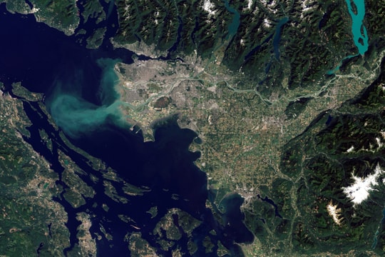
Cover image: NASA Earth Observatory image created by Robert Simmon and Jesse Allen, using Landsat data provided by the United States Geological Survey 

Fraser Floods Research Group is comprised of student researchers, Cori Hughes (BSc Earth Science), Geoffrey Niven (BA Environmental Geography), Dee Gorn (BSc Physical Geography) and Cameron Chisholm (BSc Earth Science) This study is their GEOG 455 Theoretical and Applied GIS term project to research Fraser River flooding hazards.

The individuals can be reached at the following emails:

Cameron Chisholm: cchishol@sfu.ca

Dee Gorn: deegorn.g@gmail.com

Cori Hughes: corih@sfu.ca

Geoffrey Niven: geoffniven@gmail.com