
Edge-Enhancement Filter
In Idrisi, Laplacian filters are available in three window sizes (Figure 2): 3 x 3, 5 x 5 and 7 x 7. All the landscapes of the six groups of conditions are filtered at each window size: the 120 landscapes (6 classes of 20 landscapes) will give 360 filtered images. Filters work by giving to a pixel in the resulting image a value calculated as the sum of the product of the original values within a given window. In other words, a filter multiplies the cells within a window and the sum of those products is assigned to the centre pixel (same location on a new image).
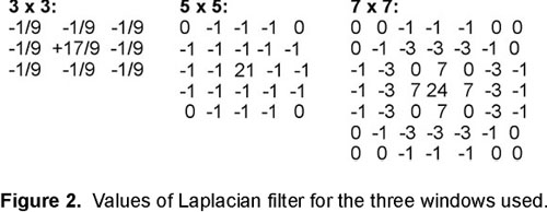
The effect of a Laplacian filter (as it is implemented in Idrisi) is to increase the difference that exists between the centre pixel and its surrounding. Figure 3 illustrates the effect of a Laplacian filter; the centre pixel is relatively higher after the filtering operation because most of the sum of the window values as been redistributed to it. Figure 4 shows the actual effect of the filter over one of the landscapes. It is obvious from this image that the filter is smoothing the image and increase only the values of the pixels that are different from their neighbours. Moreover one can see that as the window size increases, the boundary is more easily identifiable, especially on Figure 4c) and Figure 4d) where both regions have been similarly smoothed.


Slopes
In order to assess the importance of the difference in value (rate of change) between adjacent pixels, the surface module was used to compute a slope. In Idrisi, the slope is computed considering only four adjacent pixels : top, bottom, right, left (eq. 1).

Hence, the cells showing the higher slope values are the pixels having a high value in relation to their neighbours. It is then possible to state that these pixels indicate more abrupt changes. In the context of boundary (edge) recognition, one is looking for abrupt changes as a clue for boundary location; the more abrupt is the slope between two pixels, the more likely it is that these pixels separate two heterogeneous regions.
In this project, it is assumed that the pixels showing the highest slope values are elements of a boundary. It is known from the original image, where the exact location is known, that the true boundary is made up of 48 pixels or boundary elements (BEs). Therefore, the 48 highest values of slope of each filtered image have been identified as BEs.
Reclassification
Using the reclass procedure, every filtered image is being reclassified in a Boolean way so that the 48 BEs are distinct from the rest of the landscape. The value of the 48th higher slope value is used as a threshold to differentiate BEs from the background; all pixels that have a value ranging from that threshold to the maximum value of the landscape’s distribution is assigned the value 1 while all the other pixels are assigned the value 0. Figure 5 shows an example of the result the reclassification of a landscape with both high and null SA (0.0, 0.9999).

Crosstabulations
Once all the landscapes are reclassified, it is possible to evaluate how well the filtering process has identified the true boundary (i.e., the boundary of the original image) by comparing the location of the BEs from the filtered landscapes with the locations of the BEs from the original image. Figure 6 illustrates the result of the crosstab procedure in Idrisi. The results can be obtain in both text file and image so that one can proceed to a visual evaluation or compute statistics. Statistics have been computed in order to obtain averages that will allow the assessment of the combined effect the window size, SA value and difference between regional averages on the boundary recognition. Considering all these parameters, the crosstabulation procedure allows one to review the number of pixels that were correctly identified as BEs in relation with the true boundary from the original image.

Distance from the True Boundary
As the only number of pixels that were found correctly might not be sufficient to assess the performance of filters and their sensitivity to the statistical parameters, the distance of each BEs from the true boundary was calculated for every filtered image. This procedure allows to obtain an average value from an image based on the definition of another image. In this particular case, the values of average distance from the true boundary were classified following the definition of BEs (location of pixels considered as BEs and not considered BEs); only the former were used for this paper. This was made possible by using the extract procedure of Idrisi after having created a distance matrix from the true boundary of the original image.
Cartographic Model


