
The basis of a successful model, for this approach, entailed determining the areas most likely affected by larger then average waves. These areas were determined based on elevation, distance from the coastline (average sea level), and the probability of being struck by the incoming waves.
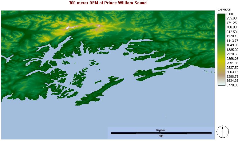
Elevation is important because it provides a major friction for water trying to move over land. Higher elevations would require the water to have significantly more energy behind it in order to raise itself up. The first step was to isolate the area of interest (Prince William Sound) from the rest of Alaska to prevent excessive computational time. By noteing the co-ordinates of the corners of the area of interest I was able to use PROJECT to trim the image down to a workable DEM.
Click on images to see a larger version.
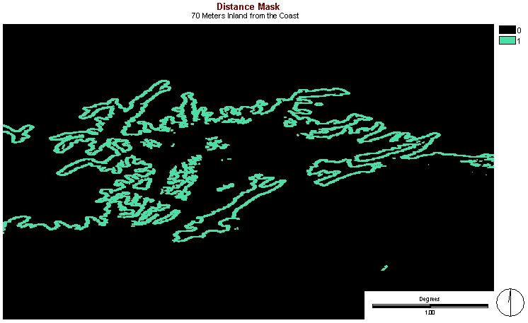
Distance is also important because water looses energy very quickly as it moves further and further inland. As it spreads inland both mass and energy are dispersed over a greater area. To create a distance surface from the DEM I created a boolean image with water as 1 and land as 0, then used COST/costgrowth to calculate the distance from the coast. To limit the display to distance water would actually be carried inland I created a boolean mask, set slightly further inland then the highest recorded distance reached by a tsunami. This was, in part, for display purposes, but also slightly reduced computational loads.


The next step was to combine distance and elevation into a weighted cost surface to determine the areas most prone to flooding (they would have the lowest cost of movement for water). In a perfect world I would have liked to use VARCOST for this because the friction would be calculated depending on the slope and direction the water was traveling in. Unfortunately, SLOPE continuously crashed on me and VARCOST wouldn't accept a substitute magnitude of friction image. An alternative was to use FUZZY on both elevation and distance to create J shaped functions, and do a weighted linear combination with elevation weighted more then distance. I chose the J-shaped function because at the coastline (elevation and distance both at 0) it would be fairly common to have slightly larger then average waves reach this point but at higher elevations, and further from shore, the likelihood that waves would reach these cells quickly drops off. Unfortunately, WEIGHT continuously crashed on me and I had to resort to the poor mans solution. I used OVERLAY to multiply elevation and distance with the reasoning that cells of higher elevation and closer to shore would have a similar value to cells of lower elevation and further from shore. I realized this would give elevation and distance equal weight but I thought water dispersing over distance might counter the weight I would have given elevation in the previous method. Finally, I standardized the resulting overlay, after masking to remove areas unlikely to be affected, to create a more easily understandable scale. 1.0 represents areas prone to flooding from tsunamis and 0.0 areas only affected by severe tsunamis.


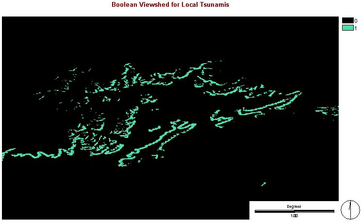
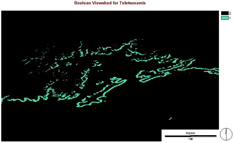
This final layer represents how the coastline would be affected if the tsunamis approached evenly. In reality this would not be the case as different parts of the coast would have different probabilities of being struck. I was unable to find on the web a model for wave behaviour (or at least one I could understand) so I thought I could approximate using VIEWSHED. I digitized two lines: one representing tsunamis generated by the fault passing through Prince William Sound and the other representing teletsunamis. If you missed it, the two types of tsunamis are defined here.


After rasterizing the lines representing the source images for the tsunamis they were used with the DEM in VIEWSHED, and masked, to create a boolean image showing areas along the coast most likely to be affected by tsunamis.
The final step, to overlay each of these with the standardized cost surface, produced the tsunami models needed to investigate the relationship between tsunamis and archeological records.


The archeological sites were digitized
as vector points by dividing them into layers based on the dates of tsunami
records. A visual inspection of the points layer on the models is
used to examine the accuracy of the model and its relavance to the investigation
of archeological sites.