Introduction
The purpose of the second portion of my
project is to analyze the spatial distribution of fire hydrants in an area
of Burnaby. The analysis was done using the Burnaby amfm data set I used
in the first part of this project. I realized, after doing the work for
the first part of my project that the hydrants provided the best opportunity
for analysis. I decided to a spatial analysis instead with the data because
the area was quite small. Doing another type of analysis, like network
analysis, did not seem logical. There was not enough information to adequately
support the analysis.
My Spatial
Question
I decided to create a project around the
spatial distribution of fire hydrants in the area. I looked at the existing
distribution of fire hydrants and I tried to determine if the current distribution
best suited the needs of the area. I will attempt to determine which structures
in the study area are well served and which are not well served. I will
also discuss two methods to solve the problem. The first is to add more
fire hydrants and the second is to determine how much additional equipment
is needed to over come a deficiency in service. This equipment would be
added to the fire trucks as needed. Insufficent acsess to fire hydrants
can cause problems for fire fighter's. I found an article on the web talking
about one situation in the South Florida area. In this situation precious
time was lost because of an improperly placed fire hydrant. View
article from the South Florida Sun Sentinel
Methodologies
The first step required me to create service
areas for each of the fire hydrants. I based my service area on the length
of a fire hose that is stretched to its full length. I also assumed that
the hose could be moved in any direction from the fire hydrant.
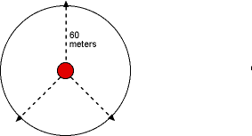
Fig 1: Service Area around the fire hydrant. The red dot represents the fire hydrants
For the purpose of my project I assumed
that a fire truck would have sixty meters of fire hose. I do not know the
accuracy of this assumption. I could not get a definite answer from those
I talked to, so I decided to take the lowest value which was sixty meters.
In this situation it seemed best to underestimate the service area rather
than over estimate. In Arcview I used the spatial analyst to define the
service area. I used the find distance command to determine the service
area. The result of this operation showed me the distance from the fire
hydrants extending out to 500 meters. All the distances were grouped using
the default classification in Arcview and were represented by a series
of colours. I used the map query command in the spatial analyst to create
the service areas. Building a query asking for all areas within 60 meters
of a fire hydrant gave me my service areas. I converted the results of
the query into a shapefile, allowing me to manipulate the information from
the query. The Shape files were used for subsequent steps in the analysis.
I overlaid the service areas with the structures
coverage. To create a coverage showing which homes are well served I used
the clip function in the geo-processing extension, it allowed me to clip
out the areas lying within the service areas. I repeated this process but
this time I selected the areas outside the service area and the structures
coverage. I used the same clip command to create a coverage containing
structures not within the service area.
Making a list of all the structures not
well served by the fire hydrants could be very useful to the fire department.
They might be interested in knowing which homes are not adequately served.
Small fires could be handled by the pumper trucks. Larger fires might require
more water and access to a fire hydrant would be needed. The residences
in this area are unique because they are generally very large and are offset
from the road. Some of the very large homes have fencing and gates which
further complicate the situation. Identifying which homes could be a problem
could allow the fire department to anticipate potential problems. Adding
a database of areas which are potential problems could allow them to be
more effective.
After I defined the service areas for the
fire hydrants and determined which structures were not being well served.
I had to find ways to solve this problem. One possible solution would be
to add additional fire hydrants in the area. To do this I created a hypothetical
criteria for locating a fire hydrant. My criteria was made up of three
factors: slope of the terrain, closeness to the road and access to water.
Locations meeting this criteria would be suitable locations for adding
a fire hydrant. This criteria is a simplistic way of looking at this problem,
I am sure there are many more factors planners take into account when they
undertake a project.
I selected slope as a selection criteria
because it would be difficult to build on steep terrain. Maintaining adequate
water pressure could also become a problem on a steep slope. Building in
steep areas could make the installation process more expensive. Visual
inspection of the fire hydrants overlaid with areas of a slope with less
than ten percent slope revealed that ten percent slope was the most inclusive.
I tried several slope values and this worked the best. I created this coverage
by making a TIN of the area from the contours coverage. This coverage includes
spot heights for points in the area. I used to the TIN to determine slope
for the area. I used the map query option to select area having a slope
less than or equal to 10%. I converted the query into a shape file.
Fire hydrants must be close to roads so
fire trucks can access them. I created a ten meter buffer around the road.
Hypothetically locations within the buffer would meet the selection criteria.
There are some problems with this concept. There are two problems with
this buffer method. When I digitized the street coverage I located the
line down the middle of the
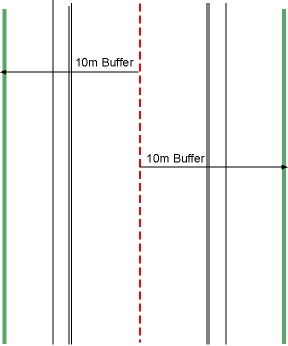
Fig 2: This represents the buffer surounding the road
The red line represent the digitized line
I added. The green lines on either side represent the far boundary of the
ten meter buffer. The black lines represent the road and the side walk.
Representing the streets this way causes a problem when I created a buffer
around the streets. The digitized line does not represent the road adequately,
it does not capture the true width of the road. I had to take this into
account when I created my buffers. I made my buffer wider to take compensate
for this. I approximated that five meters of the buffer represented the
road and the other five meters would cover the area adjacent to the road.
The final portion of my selection criteria involved access to water. I could not find out where the water mains in the area were so I used the sanitary lines coverages. Instead, I assumed that the two would be coincidental. To test this assumption I overlaid the hydrants coverage with the sanitary lines coverage. Most of the fire hydrants were within close proximity of the fire hydrants so I decided that this assumption was valid.
View 1: Fire Hydrants with Slope Less Than Ten Percent and Fire Hydrants with Sanitary Lines
To determine where the best location for fire hydrants I used the information from the three separate criteria and I combined them together. I first used the clip option in the geo-processing extension to combine the three separate coverages. I started by clipping the slope coverage with the buffer coverage. The result was a coverage showing areas inside the buffer with a slope less than ten percent. I took this newly created coverage and I used it as the input coverage for another clip command involving the sanitary lines. This final result is a coverage meeting all components of my selection criteria for locating fire hydrants.
Adding fire hydrants to the area is one
way of improving service. Another way of improving service is to improve
the equipment. In this case that would mean having more fire hoses available.
I tried to determine how additional hose would be needed to ensure that
all the area is adequately serviced. I took my initial assumption that
the service area of the fire hydrants was a circle surrounding the hydrants
with a radius of 60 meters. I expanded the service area, in ten meter increments
until all the structures were adequately covered . To do this I used the
same process I used to create the initial service areas. I preformed a
series of map queries, expanding the service area by 10 meters at a time.
When I found a service area meeting my needs I converted it into a shape
file.
Spatial
Analysis
The fire hydrants in this area follow an
irregular distribution; there is no regular spacing separating them. There
was no constancy in the spacing between each individual hydrant. I calculated
the number of fire hydrants per half square kilometer.
Fig 3: Grid representing density of fire hydrants in the area. Each grid cell represents an area .5 km squared

I placed a grid overtop of the study area.
Each square on the grid represents a half square kilometer. The areas with
the highest density are residential areas. The squares in the lower right
of the grid with values of 9,10, 8 indicates a trend of more hydrants in
residential areas. Contrast this with areas with 2,3,4,2, which are industrial
areas. This does seem to make sense; industrial and residential areas should
both have an equal number of fire hydrants. The two squares, on the bottom
right(8) and the middle right (4) are areas with very few structures but
they have a significant number of fire hydrants. I am not sure if the distribution
I found here can be found in all of Burnaby, this may only be a local trend.
Trying to take these local trends to a larger scale can result in a false
conclusion.
Based on the service areas I created there are several areas which receive poor fire hydrant service. These areas are in areas which already have a high density of hydrants per square km. These areas are in the center square( 10 per sq half kilometer) and center left (nine per square half kilometer). Infrastructure should be better organized to make for better coverage. Viewing the attribute tables for the poorly served structures and the well served structures revealed the number of poorly sered structures was about the same as the well served. There were 199 of each.
Map
of well served and poorly served areas
based
on a service areas of sixty meters
Adding more fire hydrants based on
my selection criteria would eliminate some of these gaps in service. The
result is a database which separates structures in the area into two groups,
poorly served and well served strucures. The database could be used by
by thr fire department to anicipate problems in the event of a fire. If
this was added to their dispatch system it could warn them and they could
take the appropriate action.
Map showing areas meeting all three of the selection criteria
Locating additional fire hydrants in the selected areas would solve some of these problems but there are still areas which are not adequately serviced. This could be solved by increasing the service area by making sure that the fire department has enough extra fire hose to accommodate this situation. I should also mention that there is a fire hall in this area. Areas close to the fire hall might not have to worry so much because any emergency equipment is in close proximity. My last map shows locations where I would place additional fire hydrants to improve service in the area. I also added areas where adding fire hydrants would not be practical, these areas would have to rely on a larger service area, Equipment Holdings to for firehall No.6(the only firehall in the area)
Final Map: Showing areas with additional fire hydrants and other solutions
At a distance of 130 meters all the structures were adequately serviced. This would mean an additional 70 meters of fire hose would be needed. This the distance where all the structures are serviced. Not all the fire hydrants need a service of this size to be effective. Some areas have a denser agglomeration of fire hydrants and they do not need a service area this large. The 130 meter service area is the extreme. In some locations are service area in the 100-110 meter range would be sufficient.
Map
of Service Areas with a Radius of 130 meters.
The
Structures are overlaid with on top of this coverage
Problems
The data set I used for this project represented
a small area. The area I worked with was about 2.5 sq. km. The quality
of the data that I used was very good. The data was appeared to be very
accurate, I only wish I had more data to work with. If my data covered
a greater area I believe I could of had a better project. If I had more
data I could have made stronger conclusions. With such a small data set
I found it difficult to do a relevant analysis.
Through out this project I made several
assumptions, many of these form the foundation of my analysis. The quality
of these assumptions will determine the quality of my project. The assumption
of a sixty meter service is one assumption I would like to improve. Accurate
analysis requires a number best representing the truth and I am not sure
if this number does that. Another flaw in my methodology was how I dealt
with structures on the border of the service area. If only half of a structure
is covered do I consider It well served or does the entire structure have
to be in the service area. I was not sure how to class these structures.
Converting between the grid format used
for map queries and the vector format of a shape file resulted in some
distortion. It was difficult to create circular service area from the square
grid values. The circles were jagged and not smooth like they should of
been. This jaggedness also meant that some areas that should be included
were not. This hurt the overall quality of the service areas. Another problem
caused by this transformation was that some of the lines were displaced.
After I made the transformations from the raster to vector formats I overlaid
the poorly served structures with the well served structures. The two coverages
should have lined up but they did not. To correct this problem I had to
move the points one point at a time.
The way I digitized the roads will cause
some problems, digitized roads do not truly represent the true width of
the street. Creating a problem when attempting to locate additional fire
hydrants. A portion of the buffer is actually part of the roads. Locating
fire hydrants in this area would make no sense. Finding a better way to
represent the roads would solve this problem. Digitizing the line and making
it wide enough to represent the road is one possibility. The rest of the
problems I had with this project where mostly computer problems. On two
separate occasions I had my Arcview files fail on me. Situations like this
hen are bound to happen when computers are involved. One possible solution
to this problem would be to digitize the roads as polygons, this would
better represent the demensions of the streets. To do any network analysis
I would use the roads coverage I created.
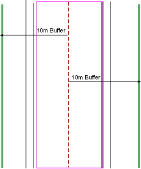
Fig 4: The area in the purple box represents
an area
which is considered in the buffer but
in reality
these areas are on the road.

Return to Index