1. Samples of students enrolled in two courses covering the same material received the following grades on their term project:
| Course A |
75.6 |
55.9 |
63.5 |
66.8 |
87.6 |
93.0 |
| 68.4 |
79.9 |
83.7 |
35.8 |
45.5 |
72.4 |
| Course B |
55.4 |
69.5 |
72.7 |
56.8 |
46.4 |
52.7 |
| 62.8 |
66.4 |
60.1 |
29.7 |
37.8 |
77.2 |
Can you conclude from this data whether the mean grade given in Course A was different from the mean grade given in Course B? Which test is appropriate to do this?
The appropriate test is the t-test for the difference between means.
a. Use the 95% level of confidence. What are your null and alternate hypotheses?

b. Is this a 1-tailed test or a 2-tailed test?
This is a 2-tailed test because the question asks if one mean is different from the other and doesn’t mention the direction of the difference.
c. What are your degrees of freedom and the critical value?

The critical value of t for a 2-tailed test at the 95% level of confidence with 22 df is 2.074.
| |
Level of significance for one-tailed test |
| .1 |
.05 |
.025 |
.01 |
.005 |
.0025 |
| df |
Level of significance for two-tailed test |
| .2 |
.1 |
.05 |
.02 |
.01 |
.005 |
| 1 |
3.078 |
6.314 |
12.706 |
31.821 |
63.657 |
127.321 |
| : |
: |
: |
: |
: |
: |
: |
| 20 |
1.325 |
1.725 |
2.086 |
2.528 |
2.845 |
3.153 |
| 21 |
1.323 |
1.721 |
2.080 |
2.518 |
2.831 |
3.135 |
| 22 |
1.321 |
1.717 |
2.074 |
2.508 |
2.819 |
3.119 |
| 23 |
1.319 |
1.714 |
2.069 |
2.500 |
2.807 |
3.104 |
| 24 |
1.318 |
1.711 |
2.064 |
2.492 |
2.797 |
3.091 |
d. Do you reject the null hypothesis?
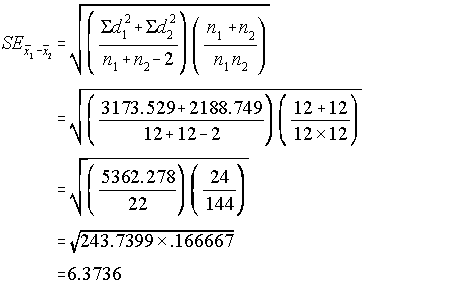
To answer this you must first calculate the modified standard error of the difference between means:


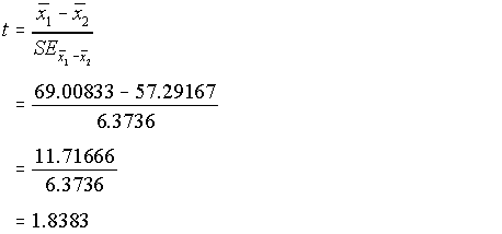
and now you can combine the modified standard error with the difference between the means to get a value for t:

Since the obtained value of t, 1.8383, is less than the critical value of 2.074, you fail to reject the null hypothesis.
e. What is your conclusion about the mean grades in the two courses?
The difference could be due to sampling variability. The difference between the two means is not statistically significant. It is possible that there is no difference overall between the grades of the students in the two courses.
2. Instead of determining whether the grades in the two courses were different, determine whether the mean grades in Course A were higher than the mean grades in Course B. Which test is appropriate?
Once again you would do a t test for the difference between means.
a. Use the 95% level of confidence. What are your null and alternate hypotheses?

b. Is this a 1-tailed test or a 2-tailed test?
It would be a 1-tailed test because the question asks about the direction of the difference and the hypotheses are directed.
c. What are your degrees of freedom and the critical value?
Because the sample sizes have not changed, the degrees of freedom are the same as for the 2-tailed test. The critical value, however, is not the same. Instead of 2.074, it is 1.717 because the second column of the table is for the 95% confidence level of 1-tailed tests.
| |
Level of significance for one-tailed test |
| .1 |
.05 |
.025 |
.01 |
.005 |
.0025 |
| df |
Level of significance for two-tailed test |
| .2 |
.1 |
.05 |
.02 |
.01 |
.005 |
| 1 |
3.078 |
6.314 |
12.706 |
31.821 |
63.657 |
127.321 |
| : |
: |
: |
: |
: |
: |
: |
| 20 |
1.325 |
1.725 |
2.086 |
2.528 |
2.845 |
3.153 |
| 21 |
1.323 |
1.721 |
2.080 |
2.518 |
2.831 |
3.135 |
| 22 |
1.321 |
1.717 |
2.074 |
2.508 |
2.819 |
3.119 |
| 23 |
1.319 |
1.714 |
2.069 |
2.500 |
2.807 |
3.104 |
| 24 |
1.318 |
1.711 |
2.064 |
2.492 |
2.797 |
3.091 |
d. Do you reject the null hypothesis?
Because the obtained value of t 1.8383, is greater than the critical value of 2.074, you reject the null hypothesis.
e. What is your conclusion about the mean grades in the two courses?
The grades of students in Course A are significantly higher than the grades of students in Course B. To say that they are “significantly” higher doesn’t mean that the difference is large; it only means that the probability of getting a difference this large due only to sampling variability is less than 5%.
3. A sample of a group of students in an evening offering of Course A received the following grades:
| Evening Course |
61.7 |
12.8 |
31.7 |
45.5 |
51.6 |
54.5 |
| 61.7 |
67.6 |
75.5 |
82.3 |
89.4 |
99.2 |
Determine whether which course the student was in is related to the mean grade awarded for the project. This requires an Analysis of Variance (ANOVA).
a. What are your hypotheses?

b. What are the degrees of freedom?
ANOVA has degrees of freedom associated with both the numerator and denominator of the F-ratio.
The degrees of freedom for the numerator, also called the between-groups df, is 2, the number of sample groups minus 1.
The degrees of freedom for the denominator, also called the within-groups df, is 33, the total number of cases in all groups (36) minus the number of groups.
c. Use the 95% confidence level. Make a summary ANOVA table like the one on page 159. Compute the Sums of Squares, Mean Squares, and the F-ratio.
| Groups |
Count |
Sum of Squares |
Mean |
Variance |
| Course A |
12 |
3173.52917 |
69.00833 |
288.50265 |
| Course B |
12 |
2188.74917 |
57.29167 |
198.97720 |
| Evening Course |
12 |
6526.68250 |
61.12500 |
593.33477 |
| Total |
36 |
11888.96083 |
|
|
| Summary ANOVA table |
| Source of Variation |
SS |
df |
MS |
F |
F-crit |
| Between Groups |
856.4867 |
2 |
428.24333 |
|
|
| Within Groups |
11888.9608 |
33 |
360.27154 |
|
|
| Total |
12745.4475 |
35 |
|
1.18867 |
3.28492 |
d. What is the critical value of F?
With 2 degrees of freedom for the numerator and 33 degrees of freedom for the denominator, the critical value at the 95% level is between 3.32 and 3.27, the numbers for 30 and 35 df. In cases like this where your df falls in between two rows of the table, the safe thing to do is to use the critical value from the row with fewer degrees of freedom than you have, rather than the value from the row with more degrees of freedom. So for this problem, you should use 3.32 as your critical value. If you are using a computer program to do the analysis for you, it will tell you the exact critical value for 2 and 33 df, which is 3.28492.
|
Critical values of F
|
|
|
Numerator degrees of freedom (p = .05 p = .01) |
| 1 |
2 |
3 |
4 |
5 |
6 |
... |
|
|
: |
: |
: |
: |
: |
: |
: |
: |
| 28 |
4.20 |
3.34 |
2.95 |
2.71 |
2.56 |
2.45 |
... |
| 7.64 |
5.45 |
4.57 |
4.07 |
3.75 |
3.53 |
... |
| 29 |
4.18 |
3.33 |
2.93 |
2.70 |
2.55 |
2.43 |
... |
| 7.60 |
5.42 |
4.54 |
4.04 |
3.73 |
3.50 |
... |
| 30 |
4.17 |
3.32 |
2.92 |
2.69 |
2.53 |
2.42 |
... |
| 7.56 |
5.39 |
4.51 |
4.02 |
3.70 |
3.47 |
... |
| 35 |
4.12 |
3.27 |
2.87 |
2.64 |
2.49 |
2.37 |
... |
| 7.42 |
5.27 |
4.40 |
3.91 |
3.59 |
3.37 |
... |
| 40 |
4.08 |
3.23 |
2.84 |
2.61 |
2.45 |
2.34 |
... |
| 7.31 |
5.18 |
4.31 |
3.83 |
3.51 |
3.29 |
... |
| : |
: |
: |
: |
: |
: |
: |
: |
e. Do you reject the null hypotheses?
Since the obtained F ratio, 1.18867, is smaller than the critical value of 3.28492, you fail to reject the null hypothesis.
f. Interpret the results of the ANOVA. You will need to compare the three means and discuss the between-groups and within-groups variances.
You can see that the mean grade for the Evening course (61.125) is in between the means for Course A (69.008) and Course B (57.292). You will remember from your answer to Question 1d and 1e that the difference between the means for Course A and Course B was not significant. It is no surprise that adding a course with a mean in between these two doesn’t result in significance.
If you look at the grades of the students in the three courses, you see that the student with the lowest grade (12.8) and the one with the highest grade (99.2) are both in the sample from the evening course. This range of grades is much larger than the range for the other two courses and there is a great deal of overlap in the range of grades for the three samples, which makes the differences between the three sample means not likely to be statistically significant.
When you look at the variance for the three samples, you see that the evening course had a much higher variance (593.335) than the other two courses (288.503 and 198.977). Since ANOVA looks at the ratio of between-groups variance (the differences between group means) and within-groups variance (the differences between members of the groups), adding the evening course sample with its high variance will increase the over all within-groups variance and will produce a low F ratio. This means that the overall differences between the three group means is not likely to be significant. If the grades of the students in the sample for the evening course had been close to one another, the result may have been quite different.
| Groups |
Mean |
Variance |
| Course A |
69.00833 |
288.50265 |
| Course B |
57.29167 |
198.97720 |
| Evening Course |
61.12500 |
593.33477 |
4. When should you do a t-test instead of a z-test?
When you have two means and the sample sizes are greater than or equal to 30, use a z-test. When you have two means and the sample sizes are smaller than 30, use a t-test. When you have more than two means, use ANOVA.
5. When should you do an F-test instead of a z-test? What can ANOVA do that the other tests for differences between means can’t do?
Both the z-test and the t-test are used to tell whether a difference between a pair of means could be due to sampling variability. They both work when the independent variable has two values — when you have two groups. If your independent variable has more than two values (if you have more than two groups), you have to use another test known as Analysis of Variance, or ANOVA.


