Multivariate Time Series Analysis

Time Series Analysis and Control Examples

Multivariate Time Series Analysis

The subroutines TSMULMAR, TSMLOMAR, and TSPRED analyze multivariate time series. The periodic AR model, TSPEARS, can also be estimated by using a vector AR procedure, since the periodic AR series can be represented as the covariance-stationary vector autoregressive model.

The stationary vector AR model is estimated and the order of the model (or each variable) is automatically determined by the minimum AIC procedure. The stationary vector AR model is written

$y_t & = & A_0 + A_1 y_{t-1} + ... + A_p y_{t-p} + \epsilon_t \\epsilon_t & \sim & N(0, \Sigma)$

Using the LDL' factorization method, the error covariance is decomposed as

$\Sigma = L{D}L^'$

where L is a unit lower triangular matrix and D is a diagonal matrix. Then the instantaneous response model is defined as

$C{y}_t = A_0^* + A_1^*y_{t-1} + ... + A_p^*y_{t-p} + \epsilon_t^*$

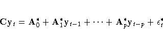
where C = L^-1, A_i^* = L^-1A_i for i = 0,1, ... ,p, and $\epsilon_t^* = L^{-1}\epsilon_t$ . Each equation of the instantaneous response model can be estimated independently, since its error covariance matrix has a diagonal covariance matrix D. Maximum likelihood estimates are obtained through the least squares method when the disturbances are normally distributed and the presample values are fixed.

The TSMULMAR call estimates the instantaneous response model. The VAR coefficients are computed using the relationship between the VAR and instantaneous models.

The general VARMA model can be transformed as an infinite order MA process under certain conditions.

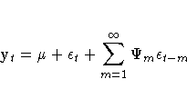
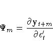
$y_t = \mu + \epsilon_t + \sum_{m=1}^{\infty} \Psi_m \epsilon_{t-m}$

In the context of the VAR(p) model, the coefficient $\Psi_m$ can be interpreted as the m-lagged response of a unit increase in the disturbances at time t.

$\Psi_m = \frac{\partial y_{t+m}}{\partial \epsilon^'_t}$

The lagged response on the one-unit increase in the orthogonalized disturbances $\epsilon_t^*$ is denoted

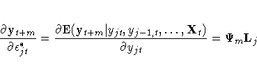
$\frac{\partial y_{t+m}}{\partial \epsilon_{jt}^*} = \frac{\partial{\rm E}(y_{t+m}| y_{jt},y_{j-1,t}, ... ,X_t)} {\partial y_{jt}} = \Psi_m L_j$

where L_j is the jth column of the unit triangular matrix L and X_t = [y_t-1, ... ,y_t-p]. When you estimate the VAR model using the TSMULMAR call, it is easy to compute this impulse response function.

The MSE of the m-step prediction is computed as

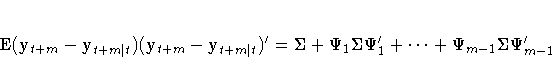
${\rm E}(y_{t+m}-y_{t+m| t})(y_{t+m}-y_{t+m| t})^' = \Sigma + \Psi_1 \Sigma \Psi^'_1 + ... + \Psi_{m-1} \Sigma \Psi^'_{m-1}$

Note that $\epsilon_t = L\epsilon_t^*$ . Then the covariance matrix of $\epsilon_t$ is decomposed

$\Sigma = \sum_{i=1}^n L_i L^'_i d_{ii}$

where d_ii is the ith diagonal element of the matrix D and n is the number of variables. The MSE matrix can be written

$\sum_{i=1}^n d_{ii} [ L_i L^'_i + \Psi_1 L_i L^'_i \Psi^'_1 + ... + \Psi_{m-1} L_i L^'_i \Psi^'_{m-1} ]$

Therefore, the contribution of the ith orthogonalized innovation to the MSE is

$V_i = d_{ii} [ L_i L^'_i + \Psi_1 L_i L^'_i \Psi^'_1 + ... + \Psi_{m-1} L_i L^'_i \Psi^'_{m-1} ]$

The ith forecast error variance decomposition is obtained from diagonal elements of the matrix V_i.

The nonstationary multivariate series can be analyzed by the TSMLOMAR subroutine. The estimation and model identification procedure is analogous to the univariate nonstationary procedure, which is explained in the "Nonstationary Time Series" section.

A time series y_t is periodically correlated with period d if Ey_t = Ey_t+d and Ey_s y_t = Ey_s+dy_t+d. Let y_t be autoregressive of period d with AR orders (p₁, ... ,p_d), that is,

$y_t = \sum_{j=1}^{p_t} \alpha_{jt}y_{t-j} + \epsilon_t$

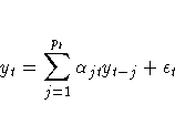
where $\epsilon_t$ is uncorrelated with mean zero and ${\rm E}\epsilon_t^2 = \sigma_t^2$ , p_t = p_t+d, $\sigma_t^2 = \sigma_{t+d}^2$ , and $\alpha_{jt} = \alpha_{j,t+d} (j=1, ... ,p_t)$ .Define the new variable such that x_jt = y_j+d(t-1). The vector series, x_t = (x_1t, ... ,x_dt)', is autoregressive of order p, where p = max_jint((p_j - j)/d) + 1. The TSPEARS subroutine estimates the periodic autoregressive model using minimum AIC vector AR modeling.

The TSPRED subroutine computes the one-step or multistep forecast of the multivariate ARMA model if the ARMA parameter estimates are provided. In addition, the subroutine TSPRED produces the (intermediate and permanent) impulse response function and performs forecast error variance decomposition for the vector AR model.

Chapter Contents
Previous
Next
Top