Editing Windows

Adding and Deleting

Many windows contain Graphs and Tables menus that enable you to add the most commonly used graphs and tables to any window. For example, in the Fit window you can add residual plots; in the Distribution window you can add tests for distributions.

If a graph you need is not listed in the Graphs menu, you can use the Analyze menu to add any graph to any window. For example, suppose you want to create a scatter plot with marginal histograms. To create this combination of graphs, first create a distribution analysis on two variables.

Choose Analyze:Distribution ( Y ).

[menu]
Figure 25.15: Analyze Menu

This displays the Distribution variables dialog.

Select GPA and HSM, then click the Y button.

This assigns GPA and HSM the Y role in the Distribution analysis.

Figure 25.16: Distribution Variables Dialog

Click the Output button.

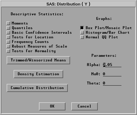
This displays the output options dialog.

In the output dialog, turn off all options except Histogram/Bar Chart.

Figure 25.17: Output Options Dialog

Click OK in both dialogs to create the distribution analysis.

Figure 25.18: Distribution Window

Now you have a distribution window with two histograms. To add a scatter plot of both variables, follow these steps.

Drag the bottom right corner of the window to the right.

This increases the window size to provide blank space to the right of the histograms.

Drag a rectangle to select an area in the window.

Figure 25.19: Area Selected

Choose Analyze:Scatter Plot ( Y X ).

This displays the scatter plot variables dialog.

In the dialog, assign GPA the Y role, and HSM the X role.

Click OK to add the scatter plot to the distribution window.

Figure 25.20: Distribution Window with Scatter Plot

You can delete any graph or table in the distribution window. For example, in this window the two small tables that contain variable names are not needed.

Click on any edge of the GPA table to select it.

Use extended selection to select the HSM table also.

Figure 25.21: Tables Selected

Choose Edit:Delete to delete the tables.

[menu]
Figure 25.22: Edit:Windows Menu

Figure 25.23: Tables Deleted

By choosing from the Analyze menu and choosing Edit:Delete, you have created a window containing one scatter plot and two histograms. In the same manner, you can add any graph and delete any graph or table in a window.

Chapter Contents
Previous
Next
Top