Chapter Contents

Previous

Next

Example 5.7: Simple Pooling Problem

The following optimization problem is discussed in Haverly (1978) and in Liebman et al. (1986, pp.127-128). Two liquid chemicals, X and Y, are produced by the pooling and blending of three input liquid chemicals, A, B, and C. You know the sulfur impurity amounts of the input chemicals, and you have to respect upper limits of the sulfur impurity amounts of the output chemicals. The sulfur concentrations and the prices of the input and output chemicals are

• Chemical A: Concentration = 3%, Price= $ 6
• Chemical B: Concentration = 1%, Price= $ 16
• Chemical C: Concentration = 2%, Price= $ 10
• Chemical X: Concentration 2.5%, Price= $ 9
• Chemical Y: Concentration 1.5%, Price= $ 15

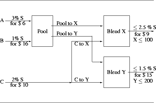
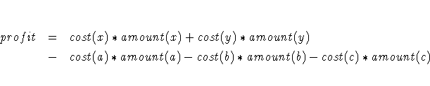
You know which customers will buy no more than 100 units of X and 200 units of Y. The problem is determining how to operate the pooling and blending of the chemicals to maximize the profit. The objective function for the profit is

There are three groups of constraints:

1. The first group of constraint functions is the mass balance restrictions illustrated by the graph. These are four linear equality constraints:
   • amount(a) + amount(b) = pool_to_x + pool_to_y
   • pool_to_x + c_to_x = amount(x)
   • pool_to_y + c_to_y = amount(y)
   • amount(c) = c_to_x + c_to_y
2. You introduce a new variable, pool_s, that represents the sulfur concentration of the pool. Using pool_s and the sulfur concentration of C (2%), you obtain two nonlinear inequality constraints for the sulfur concentrations of X and Y, one linear equality constraint for the sulfur balance, and lower and upper boundary restrictions for pool_s:
   • 
   • 
   • 3*amount(a) + 1*amount(b) = pool_s*(amount(a) + amount(b))
   • 
3. The last group assembles the remaining boundary constraints. First, you do not want to produce more than you can sell; and finally, all variables must be nonnegative:
   • ,
   • 
   • 

There exist several local optima to this problem that can be found by specifying different starting points. Using the starting point amount(a), amount(b), amount(c), amount(x), amount(y), pool_to_x, pool_to_y, c_to_x, c_to_y, pool_s, PROC NLP finds a solution with profit=400:

 proc nlp all;
  parms amountx amounty amounta amountb amountc
        pooltox pooltoy ctox ctoy pools = 1;
  bounds 0 <= amountx amounty amounta amountb amountc,
              amountx <= 100,
              amounty <= 200,
         0 <= pooltox pooltoy ctox ctoy,
         1 <= pools <= 3;
  lincon amounta + amountb = pooltox + pooltoy,
         pooltox + ctox = amountx,
         pooltoy + ctoy = amounty,
         ctox + ctoy    = amountc;
  nlincon nlc1-nlc2 >= 0.,
          nlc3 = 0.;
  max f;
  costa = 6; costb = 16; costc = 10;
  costx = 9; costy = 15;
  f = costx * amountx + costy * amounty
      - costa * amounta - costb * amountb - costc * amountc;
  nlc1 = 2.5 * amountx - pools * pooltox - 2. * ctox;
  nlc2 = 1.5 * amounty - pools * pooltoy - 2. * ctoy;
  nlc3 = 3 * amounta + amountb - pools * (amounta + amountb);
 run;

The specified starting point was not feasible with respect to the linear equality constraints; therefore, a starting point is generated that satisfies linear and boundary constraints.

 data init1(type=est);
   input _type_ $ amountx amounty amounta amountb amountc
                  pooltox pooltoy ctox ctoy pools
                  _rhs_ costa costb costc costx costy
                        ca cb cc cd;
   datalines;
     parms  1 1 1 1 1 1 1 1 1 1
            . 6 16 10 9 15  2.5 1.5 2. 3.
  ;

 proc nlp inest=init1 all;
  parms amountx amounty amounta amountb amountc
        pooltox pooltoy ctox ctoy pools;
  bounds 0 <= amountx amounty amounta amountb amountc,
              amountx <= 100,
              amounty <= 200,
         0 <= pooltox pooltoy ctox ctoy,
         1 <= pools <= 3;
  lincon amounta + amountb = pooltox + pooltoy,
         pooltox + ctox = amountx,
         pooltoy + ctoy = amounty,
         ctox + ctoy    = amountc;
  nlincon nlc1-nlc2 >= 0.,
          nlc3 = 0.;
  max f;
  f = costx * amountx + costy * amounty
      - costa * amounta - costb * amountb - costc * amountc;
  nlc1 = ca * amountx - pools * pooltox - cc * ctox;
  nlc2 = cb * amounty - pools * pooltoy - cc * ctoy;
  nlc3 = cd * amounta + amountb - pools * (amounta + amountb);
 run;

The third specification uses an INEST= data set containing the boundary and linear constraints in addition to the values of the starting point and of the constants. This specification also writes the model specification into an OUTMOD= data set:

 data init2(type=est);
   input _type_ $ amountx amounty amounta amountb amountc
                  pooltox pooltoy ctox ctoy pools
                  _rhs_ costa costb costc costx costy;
   datalines;
     parms      1   1  1  1  1    1   1   1  1  1
                .   6 16 10  9   15 2.5 1.5  2  3
     lowerbd    0   0  0  0  0    0   0   0  0  1
                .   .  .  .  .    .   .   .  .  .
     upperbd  100 200  .  .  .    .   .   .  .  3
                .   .  .  .  .    .   .   .  .  .
     eq         .   .  1  1  .   -1  -1   .  .  .
                0   .  .  .  .    .   .   .  .  .
     eq         1   .  .  .  .   -1   .  -1  .  .
                0   .  .  .  .    .   .   .  .  .
     eq         .   1  .  .  .    .  -1   . -1  .
                0   .  .  .  .    .   .   .  .  .
     eq         .   .  .  .  1    .   .  -1 -1  .
                0   .  .  .  .    .   .   .  .  .
  ;

 proc nlp inest=init2 outmod=model all;
  parms amountx amounty amounta amountb amountc
        pooltox pooltoy ctox ctoy pools;
  nlincon nlc1-nlc2 >= 0.,
          nlc3 = 0.;
  max f;
  f = costx * amountx + costy * amounty
      - costa * amounta - costb * amountb - costc * amountc;
  nlc1 = 2.5 * amountx - pools * pooltox - 2. * ctox;
  nlc2 = 1.5 * amounty - pools * pooltoy - 2. * ctoy;
  nlc3 = 3 * amounta + amountb - pools * (amounta + amountb);
 run;

The fourth specification not only reads the INEST=INIT2 data set, it also uses the model specification from the MODEL data set that was generated in the last specification. The PROC NLP call now contains only the defining variable statements:

 proc nlp inest=init2 model=model all;
  parms amountx amounty amounta amountb amountc
        pooltox pooltoy ctox ctoy pools;
  nlincon nlc1-nlc2 >= 0.,
          nlc3 = 0.;
  max f;
 run;

All four specifications start with the same starting point amount(a), amount(b), amount(c), amount(x), amount(y), pool_to_x, pool_to_y, c_to_x, c_to_y, pool_s and generate the same results. However, there exist several local optima to this problem, as is pointed out in Liebman et al. (1986, p.130).

 proc nlp inest=init2 model=model all;
  parms amountx amounty amounta amountb amountc
        pooltox pooltoy ctox ctoy = 0,
        pools = 2;
  nlincon nlc1-nlc2 >= 0.,
          nlc3 = 0.;
  max f;
 run;

This starting point is accepted as a local solution with profit=0, which, however, minimizes the profit.

Chapter Contents

Previous

Next

Top

Copyright © 1999 by SAS Institute Inc., Cary, NC, USA. All rights reserved.