Computational Formulas
The following calculations are shown for each
population and then for all populations combined.
|
Source
|
Formula
|
Dimension
|
| Probability Estimates |
| jth response | pij = [(nij)/(ni)] | 1 ×1 |
| ith population | ![p_i = [
p_{i1} \ p_{i2} \ \vdots \ p_{ir} \]](images/cateq53.gif) | r ×1 |
| all populations | ![p = [
p_1 \ p_2 \ \vdots \ p_s \]](images/cateq54.gif) | sr ×1 |
| Variance of Probability Estimates |
| ith population | Vi = [1/(ni)] (DIAG(pi) - pi pi') | r ×r |
| all populations | V = DIAG(V1, V2, ... , Vs ) | sr ×sr |
| Response Functions |
|
ith population | Fi = F(pi) | q ×1 |
| all populations | ![F = [
F_1 \ F_2 \ \vdots \ F_s \]](images/cateq55.gif) | sq ×1 |
| Derivative of Function with Respect
to Probability Estimates |
| ith population |  | q ×r |
| all populations | H = DIAG(H1, H2, ... , Hs ) | sq ×sr |
| Variance of Functions |
|
ith population | Si = Hi Vi Hi' | q ×q |
| all populations | S = DIAG(S1, S2, ... , Ss ) | sq ×sq |
| Inverse Variance of Functions |
|
ith population | Si = (Si)-1 | q ×q |
| all populations | S-1 = DIAG(S1, S2, ... , Ss ) | sq ×sq |
Derivative Table for Compound Functions: Y=F(G(p))
In the following table, let G(p) be a
vector of functions of p, and let D
denote  , which is the first
derivative matrix of G with respect to p.
, which is the first
derivative matrix of G with respect to p.
|
Function
|
Y = F(G)
|
Derivative 
|
| Multiply matrix | Y = A*G | A*D |
| Logarithm | Y = LOG(G) | DIAG-1(G)*D |
| Exponential | Y = EXP(G) | DIAG(Y)*D |
| Add constant | Y = G + A | D |
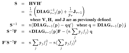
Default Response Functions: Generalized Logits
In the following table, subscripts i for the population are suppressed.
Also denote fj = log( [(pj)/(pr)] )
for j = 1, ... , r-1
for each population i = 1, ... , s.
| Inverse of Response Functions for a Population |
 |
| Form of F and Derivative for a Population |
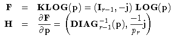 |
| Covariance Results for a Population |
 |
The following calculations are shown for each
population and then for all populations combined.
|
Source
|
Formula
|
Dimension
|
| Design Matrix |
|
ith population | Xi | q ×d |
| all populations | ![X = [
X_1 \ X_2 \ \vdots \ X_s \]](images/cateq62.gif) | sq ×d |
| Crossproduct of Design Matrix |
| ith population | Ci = Xi' Si Xi | d ×d |
| all populations | 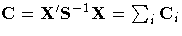 | d ×d |
| Crossproduct of Design Matrix
with Function |
| | 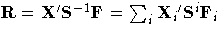 | d ×1 |
| Weighted Least-Squares Estimates |
| |
b = C-1 R = (X' S-1 X)-1 (X' S-1 F) | d ×1 |
| Covariance of
Weighted Least-Squares Estimates |
| | COV(b) = C-1 | d ×d |
| Predicted Response Functions |
| |  | sq ×1 |
| Covariance of Predicted Response Functions |
| |  | sq ×sq |
| Residual Chi-Square |
| | RSS 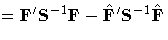 | 1 ×1 |
Chi-Square for  |
| | Q = (Lb)' (LC-1 L')-1 (Lb) | 1 ×1 |
Maximum Likelihood Method
Let C be the Hessian matrix and G be the
gradient of the log-likelihood function (both functions
of  and the parameters
  ).
Let pi* denote the vector containing the first
r-1 sample proportions from population i, and let
).
Let pi* denote the vector containing the first
r-1 sample proportions from population i, and let
 denote the corresponding vector of
probability estimates from the current iteration.
Starting with the least-squares estimates b0 of
(if you use the ML and WLS options; with the ML
option alone, the procedure starts with 0),
the probabilities
denote the corresponding vector of
probability estimates from the current iteration.
Starting with the least-squares estimates b0 of
(if you use the ML and WLS options; with the ML
option alone, the procedure starts with 0),
the probabilities  are computed,
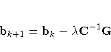
and b is calculated iteratively by the
Newton-Raphson method until it converges (see
the EPSILON= option).
The factor
are computed,
and b is calculated iteratively by the
Newton-Raphson method until it converges (see
the EPSILON= option).
The factor  is a step-halving factor that
equals one at the start of each iteration.
For any iteration in which the likelihood
decreases, PROC CATMOD uses a series of subiterations
in which is iteratively divided by two.
The subiterations continue until the likelihood
is greater than that of the previous iteration.
If the likelihood has not reached that point
after ten subiterations, then convergence is
assumed, and a warning message is displayed.
is a step-halving factor that
equals one at the start of each iteration.
For any iteration in which the likelihood
decreases, PROC CATMOD uses a series of subiterations
in which is iteratively divided by two.
The subiterations continue until the likelihood
is greater than that of the previous iteration.
If the likelihood has not reached that point
after ten subiterations, then convergence is
assumed, and a warning message is displayed.
Sometimes, infinite parameters may be present in the model, either
because of the presence of one or more zero frequencies or because
of a poorly specified model with collinearity among the estimates.
If an estimate is tending toward infinity, then PROC CATMOD
flags the parameter as infinite and holds the estimate
fixed in subsequent iterations. PROC CATMOD regards a
parameter to be infinite when two conditions apply:
- The absolute value of its estimate exceeds five
divided by the range of the corresponding variable.
- The standard error of its estimate is at least three
times greater than the estimate itself.
The estimator of the asymptotic covariance matrix of
the maximum likelihood predicted probabilities is
given by Imrey, Koch, and Stokes (1981, eq. 2.18).
The following equations summarize the method:
where
![C & = & X{'}S^{-1}({\pi}) {X } \
N & = & [ n_1 ( p_1^* - {\pi}_1^* ) \ \vdots \n_s ( p_s^* - {\pi}_s^* ) \ ] \
& & \G & = & X{'}N \](images/cateq72.gif)
Copyright © 1999 by SAS Institute Inc., Cary, NC, USA. All rights reserved.