Tests and Measures of Agreement

The FREQ Procedure

Tests and Measures of Agreement

When you specify the AGREE option in the TABLES statement, PROC FREQ computes tests and measures of agreement for square tables (that is, for tables where the number of rows equals the number of columns). For two-way tables, these tests and measures include McNemar's test for 2 ×2 tables, Bowker's test of symmetry, the simple kappa coefficient, and the weighted kappa coefficient. For multiple strata (n-way tables, where n > 2), PROC FREQ computes the overall simple kappa coefficient and the overall weighted kappa coefficient, as well as tests for equal kappas (simple and weighted) among strata. Cochran's Q is computed for multi-way tables when each variable has two levels, that is, for 2 ×2 ×... ×2 tables.

PROC FREQ computes the kappa coefficients (simple and weighted), their asymptotic standard errors, and their confidence limits when you specify the AGREE option in the TABLES statement. If you also specify the KAPPA option in the TEST statement, then PROC FREQ computes the asymptotic test of the hypothesis that simple kappa equals zero. Similarly, if you specify the WTKAP option in the TEST statement, PROC FREQ computes the asymptotic test for weighted kappa.

In addition to the asymptotic tests described in this section, PROC FREQ computes the exact p-value for McNemar's test when you specify the option MCNEM in the EXACT statement. For the kappa statistics, PROC FREQ computes the exact test of the hypothesis that kappa (or weighted kappa) equals zero when you specify the option KAPPA (or WTKAP) in the EXACT statement. See the section "Exact Statistics" for information on exact tests.

The discussion of each test and measures of agreement provides the formulas that PROC FREQ uses to compute the AGREE statistics. For information on the use and interpretation of these statistics, refer to Agresti (1990), Agresti (1996), Fleiss (1981), and the other references cited for each statistic.

McNemar's Test

PROC FREQ computes McNemar's test for 2 ×2 tables when you specify the AGREE option. McNemar's test is appropriate when you are analyzing data from matched pairs of subjects with a dichotomous (yes-no) response. It tests the null hypothesis of marginal homogeneity, or p_{1 ·} = p_·1. McNemar's test is computed as

Q_M = [((n₁₂-n₂₁)²)/(n₁₂+n₂₁)]

Under the null hypothesis, Q_M has an asymptotic chi-square distribution with one degree of freedom. Refer to McNemar (1947), as well as the references cited in the preceding section. In addition to the asymptotic test, PROC FREQ also computes the exact p-value for McNemar's test when you specify the MCNEM option in the EXACT statement.

Bowker's Test of Symmetry

For Bowker's test of symmetry, the null hypothesis is that the probabilities in the square table satisfy symmetry or that p_ij = p_ji for all pairs of table cells. When there are more than two categories, Bowker's test of symmetry is calculated as

$Q_{B} = \raisebox{-2ex}{\stackrel{\displaystyle\sum \! \displaystyle\sum} {\scriptstyle i \lt j}}\frac{(n_{ij}-n_{ji})^2}{n_{ij}+n_{ji}}$

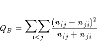
For large samples, Q_B has an asymptotic chi-square distribution with R(R-1)/2 degrees of freedom under the null hypothesis of symmetry of the expected counts. Refer to Bowker (1948). For two categories, this test of symmetry is identical to McNemar's test.

Simple Kappa Coefficient

The simple kappa coefficient, introduced by Cohen (1960), is a measure of interrater agreement:

$\hat{\kappa} = \frac{P_o - P_e}{1-P_e}$

where $P_o = \sum_i p_{ii}$ and $P_e = \sum_i p_{i.} p_{.i}$ .If the two response variables are viewed as two independent ratings of the n subjects, the kappa coefficient equals +1 when there is complete agreement of the raters. When the observed agreement exceeds chance agreement, kappa is positive, with its magnitude reflecting the strength of agreement. Although this is unusual in practice, kappa is negative when the observed agreement is less than chance agreement. The minimum value of kappa is between -1 and 0, depending on the marginal proportions.

The asymptotic variance of the simple kappa coefficient can be estimated by the following, according to Fleiss, Cohen, and Everitt (1969):

var = [(A + B - C)/((1-P_e)²n)]

where

$A = \sum_i p_{ii} \biggl[ 1-(p_{i \cdot} + p_{\cdot i})(1-\hat{\kappa})\biggr]^2$

$B = (1-\hat{\kappa})^2 \raisebox{-2ex}{\stackrel{\displaystyle\sum \! \displaystyle\sum} {\scriptstyle i \neq j}} p_{ij} (p_{\cdot i} + p_{j \cdot})^2$

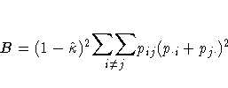
and

$C = \biggl[ \hat{\kappa} - P_e (1-\hat{\kappa})\biggr]^2$

PROC FREQ computes confidence limits for the simple kappa coefficient according to

$\hat{\kappa} +- z_{\alpha/2} \cdot \sqrt{var}$

where $z_{\alpha/2}$ is the $100(1 - \alpha/2)$ percentile of the standard normal distribution. The value of $\alpha$ is determined by the value of the ALPHA= option, which, by default, equals 0.05 and produces 95% confidence limits.

To compute an asymptotic test for the kappa coefficient, PROC FREQ uses a standardized test statistic $\hat{\kappa}^\ast$ ,which has an asymptotic standard normal distribution under the null hypothesis that kappa equals zero. The standardized test statistic is computed as

$\hat{\kappa}^\ast = \frac{\hat{\kappa}} {\sqrt{var_0(\hat{\kappa})}}$

where $var_0(\hat{\kappa})$ is the variance of the kappa coefficient under the null hypothesis.

$var_0(\hat{\kappa}) = \frac{P_e + P_e^2 - \sum_i p_{i \cdot} p_{\cdot i} (p_{i \cdot} + p_{\cdot i})} {(1 - P_e)^2 n}$

Refer to Fleiss (1981).

In addition to the asymptotic test for kappa, PROC FREQ computes the exact test when you specify the KAPPA or AGREE option in the EXACT statement. See the section "Exact Statistics" for information on exact tests.

Weighted Kappa Coefficient

The weighted kappa coefficient is a generalization of the simple kappa coefficient, using weights to quantify the relative difference between categories. For 2×2 tables, the weighted kappa coefficient equals the simple kappa coefficient. PROC FREQ displays the weighted kappa coefficient only for tables larger than 2×2. PROC FREQ computes the weights from the column scores, using either the Cicchetti-Allison weight type or the Fleiss-Cohen weight type, both of which are described in the following section. The weights w_ij are constructed so that 0<=w_ij<1 for all $i \not= j$ , w_ii = 1 for all i, and w_ij = w_ji. The weighted kappa coefficient is defined as

$\hat{\kappa}_w = \frac{P_{o(w)} - P_{e(w)}}{1-P_{e(w)}}$

where

$P_{o(w)} = \sum_i \sum_j w_{ij} p_{ij}$

and

$P_{e(w)} = \sum_i \sum_j w_{ij} p_{i \cdot} p_{\cdot j}$

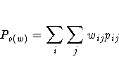
The asymptotic variance of the weighted kappa coefficient can be estimated by the following, according to Fleiss, Cohen, and Everitt (1969):

$var = \frac{\sum_i\sum_j p_{ij} \biggl[w_{ij}-(\overline{w}_{i \cdot}+\overline... ...biggl[\hat{\kappa}_w - P_{e(w)}(1-\hat{\kappa}_w)\biggr]^2} {(1-P_{e(w)})^2n}$

where

$\overline{w}_{i \cdot} = \sum_j p_{\cdot j}w_{ij}$

and

$\overline{w}_{\cdot j} = \sum_i p_{i \cdot}w_{ij}$

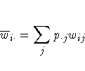
PROC FREQ computes confidence limits for the weighted kappa coefficient according to

$\hat{\kappa}_w +- z_{\alpha/2} \cdot \sqrt{var}$

To compute an asymptotic test for the weighted kappa coefficient, PROC FREQ uses a standardized test statistic $\hat{\kappa}_w^\ast$ ,which has an asymptotic standard normal distribution under the null hypothesis that weighted kappa equals zero. The standardized test statistic is computed as

$\hat{\kappa}_w^\ast = \frac{\hat{\kappa}_w} {\sqrt{var_0(\hat{\kappa}_w)}}$

where $var_0(\hat{\kappa}_w)$ is the variance of the weighted kappa coefficient under the null hypothesis.

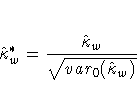
$var_0(\hat{\kappa}_w) = \frac{\sum_i \sum_j p_{i \cdot} p_{\cdot j} \biggl[ w_... ...cdot} + \overline{w}_{\cdot j}) \biggr] ^2 - P_{e(w)}^2 } {(1 - P_{e(w)})^2 n}$

Refer to Fleiss (1981).

In addition to the asymptotic test for weighted kappa, PROC FREQ computes the exact test when you specify the WTKAP or AGREE option in the EXACT statement. See the section "Exact Statistics" for information on exact tests.

Weights PROC FREQ computes kappa coefficient weights using the column scores and one of two available weight types. The column scores are determined by the SCORES= option in the TABLES statement. The two available weight types are Cicchetti-Allison and Fleiss-Cohen, and PROC FREQ uses the Cicchetti-Allison type by default. If you specify (WT=FC) with the AGREE option, then PROC FREQ uses the Fleiss-Cohen weight type to construct kappa weights.

PROC FREQ computes Cicchetti-Allison kappa coefficient weights using a form similar to that given by Cicchetti and Allison (1971).

$w_{ij} = 1 - \frac{| C_i - C_j|}{C_C - C_1}$

where C_i is the score for column i, and C is the number of categories or columns. You can specify the score type using the SCORES= option in the TABLES statement; if you do not specify the SCORES= option, PROC FREQ uses table scores. For numeric variables, table scores are the values of the numeric row and column headings. You can assign numeric values to the categories in a way that reflects their level of similarity. For example, suppose you have four categories and order them according to similarity. If you assign them values of 0, 2, 4, and 10, the following weights are used for computing the weighted kappa coefficient: w₁₂ = 0.8, w₁₃ = 0.6, w₁₄ = 0, w₂₃ = 0.8, w₂₄ = 0.2, and w₃₄ = 0.4. Note that when there are only two categories (that is, C = 2), the weighted kappa coefficient is identical to the simple kappa coefficient.

If you specify (WT=FC) with the AGREE option in the TABLES statement, PROC FREQ computes Fleiss-Cohen kappa coefficient weights using a form similar to that given by Fleiss and Cohen (1973).

w_ij = 1 - [((C_i - C_j)²)/((C_C - C₁)²)]

For the preceding example, the weights used for computing the weighted kappa coefficient are: w₁₂ = 0.96, w₁₃ = 0.84, w₁₄ = 0, w₂₃ = 0.96, w₂₄ = 0.36, and w₃₄ = 0.64.

Overall Kappa Coefficient

When there are multiple strata, PROC FREQ combines the stratum-level estimates of kappa into an overall estimate of the supposed common value of kappa. Assume there are q strata, indexed by h=1,2,...,q, and let $var(\hat{\kappa}_h)$ denote the squared standard error of $\hat{\kappa}_h$ . Then the estimate of the overall kappa, according to Fleiss (1981), is computed as

$\hat{\kappa}_{overall} = \sum_{h=1}^q \frac{\hat{\kappa}_h} {var(\hat{\kappa}_h)} / \sum_{h=1}^q \frac{1}{var(\hat{\kappa}_h)}$

An estimate of the overall weighted kappa is computed in a similar manner.

Tests for Equal Kappa Coefficients

The following chi-square statistic, with q-1 degrees of freedom, is used to test whether the values of kappa are equal among the q strata:

$Q_K = \sum_{h=1}^q \frac{(\hat{\kappa}_h - \hat{\kappa}_{overall})^2} {var(\hat{\kappa}_h)}$

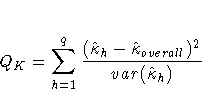
A similar test is performed for weighted kappa coefficients.

Cochran's Q Test

Cochran's Q is computed for multi-way tables when each variable has two levels, that is, for 2 ×2 ... ×2 tables. Cochran's Q statistic is used to test the homogeneity of the one-dimensional margins. Let m denote the number of variables and N denote the total number of subjects. Then Cochran's Q statistic is computed as

$Q_C = (m-1) \frac{m \sum_{j=1}^m T_j^2 - T^2} {mT - \sum_{k=1}^N S_k^2}$

where T_j is the number of positive responses for variable j, T is the total number of positive responses over all variables, and S_k is the number of positive responses for subject k. Under the null hypothesis, Cochran's Q is an approximate chi-square statistic with m-1 degrees of freedom. Refer to Cochran (1950). When there are only two binary response variables (m=2), Cochran's Q simplifies to McNemar's test. When there are more than two response categories, you can test for marginal homogeneity using the repeated measures capabilities of the CATMOD procedure.

Tables with Zero Rows and Columns

For multiway tables, PROC FREQ does not compute CHISQ or MEASURES statistics for a stratum with a zero row or a zero column, because most of these statistics are undefined in this case. For a two-way table where there is no stratification, the analysis includes only those levels that occur with nonzero weight. However, PROC FREQ does compute AGREE statistics for stratified tables with a zero row or a zero column. The analysis includes all row and column variable levels that occur in any stratum. It does not include levels that do not occur in any stratum, even if such observations are in the data set with zero weight, because PROC FREQ does not process observations with zero weights (as described in the section "WEIGHT Statement").

To include a variable level with no observations in the analysis, you can assign an extremely small weight (such as 1E-8) to an observation with that variable level. Then the analysis includes this variable level, but the statistic value remains unchanged because the weight is so small. For example, suppose you need to compute a kappa coefficient for data from two raters. One rater uses all possible ratings (say, 1, 2, 3, 4, and 5), but another rater uses only four of the available ratings (1, 2, 3, and 4). You can create an observation where the second rater uses the rating level 5 and assign it a weight of 1E-8. This forms a 5 ×5 table for the analysis.

Chapter Contents
Previous
Next
Top