MODEL Statement
- MODEL response = < effects > < /options > ;
- MODEL events/trials = < effects > < /options > ;
The MODEL statement specifies the response, or dependent
variable, and the effects, or explanatory variables.
If you omit the explanatory variables,
the procedure fits an intercept-only model.
An intercept term is included in the model by default.
The intercept can be removed with the NOINT option.
You can specify the response in the form of a single
variable or in the form of a ratio of two variables denoted
events/trials.
The first form is applicable
to all responses.
The second form is applicable only to summarized binomial response data.
When each observation in the input data set contains the number of
events (for example, successes) and the number of trials from a set
of binomial trials, use the events/trials syntax.
In the events/trials model syntax,
you specify two variables that contain
the event and trial counts.
These two variables are separated by a slash (/).
The values of both events and (trials-events)
must be nonnegative, and the value of the trials variable
must be greater than 0 for an observation to be valid.
The variable events or trials may take noninteger values.
When each observation in the input data set contains a single trial
from a binomial or multinomial experiment, use the first form of the
MODEL statement above. The response variable can be numeric or character.
The ordering of response levels is critical in these models. You can
use the RORDER= option in the PROC GENMOD statement to specify the response level ordering.
Responses for the Poisson distribution must be
positive, but they can be noninteger values.
The effects in the MODEL statement consist of
an explanatory variable or combination of variables.
Explanatory variables can be
continuous or classification variables.
Classification variables can be character or numeric.
Explanatory variables representing nominal, or
classification, data must be declared in a CLASS statement.
Interactions between variables can also be included as effects.
Columns of the design matrix are automatically
generated for classification variables and interactions.
The syntax for specification of effects
is the same as for the GLM procedure.
See the "Specification of Effects" section for more information.
Also refer to Chapter 30, "The GLM Procedure."
You can specify the following options in
the MODEL statement after a slash (/).
- AGGREGATE= (variable-list)
- AGGREGATE= variable
-
specifies the subpopulations
on which the Pearson chi-square
and the deviance
are calculated. This option applies only to the multinomial
distribution or the binomial distribution with binary
(single trial syntax) response. It is ignored if
specified for other cases.
Observations with common values
in the given list of variables are regarded as coming from
the same subpopulation. This affects the computation of
the deviance and Pearson chi-square statistics.
Variables in the list can be any variables in the input data set.
- ALPHA | ALPH | A=number
-
sets the confidence coefficient
for parameter confidence intervals to 1-number.
The value of number must be between 0 and 1.
The default value of number is 0.05.
- CICONV=number
-
sets the convergence criterion for
profile likelihood confidence intervals.
See the section "Confidence Intervals for Parameters" for the definition of convergence.
The value of number must be between 0 and 1.
By default, CICONV=1E-4.
- CL
-
requests that confidence limits for predicted values
be displayed. See the OBSTATS option.
- CONVERGE=number
-
sets the convergence criterion
.
The value of number must be between 0 and 1.
The iterations are considered to have converged when
the maximum change in the parameter estimates between
iteration steps is less than the value specified.
The change is a relative change if the parameter is greater than
0.01 in absolute value; otherwise, it is an absolute change.
By default, CONVERGE=1E-4.
This convergence criterion is used in parameter estimation
for a single model fit, Type 1 statistics, and likelihood
ratio statistics for Type 3 analyses and CONTRAST statements.
- CONVH=number
-
sets the relative Hessian convergence criterion.
The value of number must be between 0 and 1.
After convergence is
determined with the change in parameter criterion
specified with the CONVERGE= option, the quantity
 is computed and compared to
number, where g is the gradient vector, H is the
Hessian matrix for the model parameters, and f is the log-likelihood
function. If tc is greater than
number, a warning that the relative Hessian convergence criterion
has been exceeded is printed.
This criterion detects the occasional case where the change in parameter
convergence criterion is satisfied, but a maximum in the log-likelihood
function has not been attained.
By default, CONVH=1E-4.
is computed and compared to
number, where g is the gradient vector, H is the
Hessian matrix for the model parameters, and f is the log-likelihood
function. If tc is greater than
number, a warning that the relative Hessian convergence criterion
has been exceeded is printed.
This criterion detects the occasional case where the change in parameter
convergence criterion is satisfied, but a maximum in the log-likelihood
function has not been attained.
By default, CONVH=1E-4.
- CORRB
-
requests that the parameter estimate correlation
matrix be displayed.
- COVB
-
requests that the parameter estimate covariance matrix
be displayed.
- DIST | D | ERROR | ERR = keyword
-
specifies the built-in probability distribution
to use in the model.
If you specify the DIST= option and you omit a
user-defined link function, a default link
function is chosen as displayed in the following table.
If you specify no distribution and no link function,
then the GENMOD procedure defaults to the normal
distribution with the identity link function.
|
DIST=
|
Distribution
|
Default Link Function
|
| BINOMIAL | BIN | B | binomial | logit |
| GAMMA | GAM | G | gamma | inverse ( power(-1) ) |
| IGAUSSIAN | IG | inverse Gaussian | inverse squared ( power(-2) ) |
| MULTINOMIAL | MULT | multinomial | cumulative logit |
| NEGBIN | NB | negative binomial | log |
| NORMAL | NOR | N | normal | identity |
| POISSON | POI | P | Poisson | log |
- EXPECTED
-
requests that the expected Fisher information
matrix be used to compute parameter estimate
covariances and the associated statistics.
The default action is to use the
observed Fisher information matrix. See the SCORING= option.
- ID=variable
- causes the values of variable
in the input data set to be displayed in the OBSTATS table.
If an explicit format for variable has been defined, the formatted
values are displayed. If the OBSTATS option is not specified, this option has
no effect.
- INITIAL=numbers
-
sets initial values
for parameter estimates in the model.
The default initial parameter values are weighted
least squares estimates based on using the
response data as the initial mean estimate.
This option can be useful in case of convergence difficulty.
The intercept parameter is initialized with
the INTERCEPT= option and is not included here.
The values are assigned to the variables in the MODEL statement
in the same order in which they appear in the MODEL statement.
The order of levels for CLASS variables
is determined by the ORDER= option.
Note that some levels of class variables can be
aliased; that is, they correspond to linearly dependent
parameters that are not estimated by the procedure.
Initial values must be assigned to all levels of class
variables, regardless of whether they are aliased or not.
The procedure ignores initial values
corresponding to parameters not being estimated.
If you specify a BY statement, all class variables must
take on the same number of levels in each BY group.
Otherwise, class variables in some of the BY
groups are assigned incorrect initial values.
Types of INITIAL= specifications are
illustrated in the following table.
|
Type of List
|
Specification
|
| list separated by blanks | INITIAL = 3 4 5 |
| list separated by commas | INITIAL = 3, 4, 5 |
| x to y | INITIAL = 3 to 5 |
| x to y by z | INITIAL = 3 to 5 by 1 |
| combination of list types | INITIAL = 1, 3 to 5, 9 |
- INTERCEPT=number
-
initializes the intercept term to
number for parameter estimation.
If you specify both the INTERCEPT= and the NOINT options,
the intercept term is not estimated, but
an intercept term of number is included in the model.
- ITPRINT
-
displays the iteration history for all iterative processes:
parameter estimation, fitting constrained models for contrasts
and Type 3 analyses, and profile likelihood confidence intervals.
The last evaluation of the gradient and the
negative of the Hessian (second derivative)
matrix are also displayed for parameter estimation.
This option may result in a large amount of
displayed output, especially if some of the
optional iterative processes are selected.
- LINK = keyword
-
specifies the link function
to use in the model.
The keywords and their associated
built-in link functions are as follows.
|
LINK=
|
Link Function
|
| CUMCLL | CCLL | cumulative complementary log-log |
| CUMLOGIT | CLOGIT | cumulative logit |
| CUMPROBIT | CPROBIT | cumulative probit |
| CLOGLOG | CLL | complementary log-log |
| IDENTITY | ID | identity |
| LOG | log |
| LOGIT | logit |
| PROBIT | probit |
| POWER(number) | POW(number) | power with  =
number =
number |
If no LINK= option is supplied and there is a user-defined
link function, the user-defined link function is used.
If you specify neither the LINK= option nor a user-defined link
function, then the default canonical link
function is used if you specify the DIST= option.
Otherwise, if you omit the DIST= option,
the identity link function is used.
The cumulative link functions are appropriate only
for the multinomial distribution.
- LRCI
-
requests that two-sided confidence intervals for all model
parameters be computed based on the profile likelihood function.
This is sometimes called the partially
maximized likelihood function.
See the "Confidence Intervals for Parameters" section for more
information on the profile likelihood function.
This computation is iterative and can consume
a relatively large amount of CPU time.
The confidence coefficient can be selected
with the ALPHA=number option.
The resulting confidence coefficient is 1-number.
The default confidence coefficient is 0.95.
- MAXITER=number
- MAXIT=number
-
sets the maximum allowable number of iterations for
all iterative computation processes in PROC GENMOD.
By default, MAXITER=50.
- NOINT
-
requests that no intercept term
be included in the model.
An intercept is included unless this option is specified.
- NOSCALE
-
holds the scale parameter fixed.
Otherwise, for the normal, inverse gaussian,
and gamma distributions, the scale parameter
is estimated by maximum likelihood.
If you omit the
SCALE= option, the
scale parameter is fixed at the value 1.
- OFFSET=variable
-
specifies a variable in the input data set to be used as an offset
variable.
This variable cannot be a CLASS variable, and it cannot be
the response variable or one of the explanatory variables.
- OBSTATS
-
specifies that an additional table of statistics be displayed.
For each observation, the following items are displayed:
- the value of the response variable
(variables if the data are binomial),
frequency, and weight variables
- the values of the regression variables
- predicted mean,
 , where
  is the linear
predictor and g is the link function.
If there is an offset, it is included in
is the linear
predictor and g is the link function.
If there is an offset, it is included in  .
. - estimate of the linear predictor . If there is an offset, it is included in .
- standard error of the linear predictor
- the value of the Hessian weight at the final iteration
- lower confidence limit of the predicted value of the mean.
The confidence coefficient is
specified with the ALPHA= option.
See the section "Confidence Intervals on Predicted Values" for the computational method.
- upper confidence limit of the predicted value of the mean
- raw residual, defined as

- Pearson, or chi residual, defined as the square root
of the contribution for the observation to the Pearson
chi-square, that is
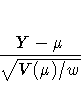
where Y is the response,  is the predicted mean,
w is the value of the prior weight variable specified
in a WEIGHT statement, and V() is the variance
function evaluated at .
is the predicted mean,
w is the value of the prior weight variable specified
in a WEIGHT statement, and V() is the variance
function evaluated at . - the standardized Pearson residual
- deviance residual, defined as the square root of the
deviance contribution for the observation, with sign
equal to the sign of the raw residual
- the standardized deviance residual
- the likelihood residual
The RESIDUALS, PREDICTED, XVARS, and CL options cause only
subgroups of the observation statistics to be displayed. You
can specify more than one of these options to include
different subgroups of statistics.
The ID=variable option causes the values of variable
in the input data set to be displayed in the table. If an explicit format for
variable has been defined, the formatted values are displayed.
If a REPEATED statement is present, a table is displayed for the
GEE model specified in the REPEATED statement. Only
the regression variables, response values, predicted values,
confidence limits for the predicted values, linear predictor,
raw residuals, and Pearson residuals for each observation in the
input data set are available.
- PREDICTED
- PRED
- P
-
requests that predicted values, the linear predictor, its
standard error, and the Hessian weight be displayed.
See the OBSTATS option.
- RESIDUALS
- R
-
requests that residuals and standardized residuals be displayed.
See the OBSTATS option.
- SCALE=number
- SCALE=PEARSON
- SCALE=P
- PSCALE
- SCALE=DEVIANCE
- SCALE=D
- DSCALE
-
sets the value used for the scale
parameter where the NOSCALE option is used.
For the binomial and Poisson distributions,
which have no free scale parameter, this can
be used to specify an overdispersed model.
In this case, the parameter covariance matrix and the
likelihood function are adjusted by the scale parameter.
See the "Dispersion Parameter" section and the "Overdispersion" section
for more information.
If the NOSCALE option is not specified, then number
is used as an initial estimate of the scale parameter.
Specifying SCALE=PEARSON or SCALE=P is the same as specifying the PSCALE option.
This fixes the scale parameter at the
value 1 in the estimation procedure.
After the parameter estimates are determined, the
exponential family dispersion parameter is assumed to be given
by Pearson's chi-square statistic divided by the degrees
of freedom, and all statistics such as standard errors and
likelihood ratio statistics are adjusted appropriately.
Specifying SCALE=DEVIANCE or SCALE=D is the same as specifying the DSCALE option.
This fixes the scale parameter at a value
of 1 in the estimation procedure.
After the parameter estimates are determined, the
exponential family dispersion parameter is assumed to be
given by the deviance divided by the degrees of freedom.
All statistics such as standard errors and likelihood
ratio statistics are adjusted appropriately.
- SCORING=number
-
requests that on iterations up to number, the Hessian
matrix is computed using the Fisher's scoring method.
For further iterations, the full Hessian matrix is computed.
The default value is 1.
A value of 0 causes all iterations to use the full
Hessian matrix, and a value greater than or equal to the
value of the MAXITER option causes all iterations to use Fisher's scoring.
The value of the SCORING= option must be 0 or a positive integer.
- SINGULAR=number
-
sets the tolerance for testing singularity
of the information matrix and the crossproducts matrix.
Roughly, the test requires that a pivot be at least
this number times the original diagonal value.
By default, number is 107 times the machine epsilon.
The default number is
approximately 10-9 on most machines.
- TYPE1
-
requests that a Type 1, or sequential, analysis be performed.
This consists of sequentially fitting models, beginning
with the null (intercept term only) model and continuing
up to the model specified in the MODEL statement.
The likelihood ratio statistic between each successive
pair of models is computed and displayed in a table.
A Type 1 analysis is not available for GEE models,
since there is no associated likelihood.
- TYPE3
-
requests that statistics for Type 3 contrasts be computed
for each effect specified in the MODEL statement.
The default analysis is to compute likelihood
ratio statistics for the contrasts or score
statistics for GEEs.
Wald statistics are computed if
the WALD option is also specified.
- WALD
-
requests Wald statistics for Type 3 contrasts.
You must also specify the TYPE3 option in
order to compute Type 3 Wald statistics.
- WALDCI
-
requests that two-sided Wald confidence intervals
for all model parameters be computed based on the
asymptotic normality of the parameter estimators.
This computation is not as time consuming as the LRCI
method, since it does not involve an iterative procedure.
However, it is not thought to be as
accurate, especially for small sample sizes.
The confidence coefficient can be selected with the
ALPHA= option in the same way as for the LRCI option.
- XVARS
-
requests that the regression variables be included in the
OBSTATS table.
Copyright © 1999 by SAS Institute Inc., Cary, NC, USA. All rights reserved.