The LOGISTIC Procedure

Overview

Binary responses (for example, success and failure) and ordinal responses (for example, normal, mild, and severe) arise in many fields of study. Logistic regression analysis is often used to investigate the relationship between these discrete responses and a set of explanatory variables. Several texts that discuss logistic regression are Collett (1991), Agresti (1990), Cox and Snell (1989), and Hosmer and Lemeshow (1989).

For binary response models, the response, Y, of an individual or an experimental unit can take on one of two possible values, denoted for convenience by 1 and 2 (for example, Y=1 if a disease is present, otherwise Y=2). Suppose x is a vector of explanatory variables and $p=\Pr({\rm Y}=1|{x})$ is the response probability to be modeled. The linear logistic model has the form

${logit}(p) \equiv \log (\frac{p}{1-p})= \alpha + {\beta}'x$

where $\alpha$ is the intercept parameter and ${\beta}$ is the vector of slope parameters. Notice that the LOGISTIC procedure, by default, models the probability of the lower response levels.

The logistic model shares a common feature with a more general class of linear models, that a function $g=g(\mu)$ of the mean of the response variable is assumed to be linearly related to the explanatory variables. Since the mean $\mu$ implicitly depends on the stochastic behavior of the response, and the explanatory variables are assumed to be fixed, the function g provides the link between the random (stochastic) component and the systematic (deterministic) component of the response variable Y. For this reason, Nelder and Wedderburn (1972) refer to $g(\mu)$ as a link function. One advantage of the logit function over other link functions is that differences on the logistic scale are interpretable regardless of whether the data are sampled prospectively or retrospectively (McCullagh and Nelder 1989, Chapter 4). Other link functions that are widely used in practice are the probit function and the complementary log-log function. The LOGISTIC procedure enables you to choose one of these link functions, resulting in fitting a broader class of binary response models of the form

$g(p)=\alpha + {\beta}' x$

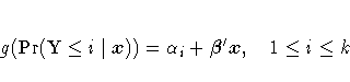
For ordinal response models, the response, Y, of an individual or an experimental unit may be restricted to one of a (usually small) number, $k+1 (k \ge 1 )$ , of ordinal values, denoted for convenience by 1, ... ,k, k+1. For example, the severity of coronary disease can be classified into three response categories as 1=no disease, 2=angina pectoris, and 3=myocardial infarction. The LOGISTIC procedure fits a common slopes cumulative model, which is a parallel lines regression model based on the cumulative probabilities of the response categories rather than on their individual probabilities. The cumulative model has the form

$g(\Pr({\rm Y} \le i|{x}))= \alpha_i + {\beta}' x , 1 \le i \le k$

where $\alpha_1, ... ,\alpha_{k}$ are k intercept parameters, and ${\beta}$ is the vector of slope parameters. This model has been considered by many researchers. Aitchison and Silvey (1957) and Ashford (1959) employ a probit scale and provide a maximum likelihood analysis; Walker and Duncan (1967) and Cox and Snell (1989) discuss the use of the log-odds scale. For the log-odds scale, the cumulative logit model is often referred to as the proportional odds model.

The LOGISTIC procedure fits linear logistic regression models for binary or ordinal response data by the method of maximum likelihood. The maximum likelihood estimation is carried out with either the Fisher-scoring algorithm or the Newton-Raphson algorithm. You can specify starting values for the parameter estimates. The logit link function in the logistic regression models can be replaced by the probit function or the complementary log-log function.

The LOGISTIC procedure provides four variable selection methods: forward selection, backward elimination, stepwise selection, and best subset selection. The best subset selection is based on the likelihood score statistic. This method identifies a specified number of best models containing one, two, three variables and so on, up to a single model containing all the explanatory variables.

Odds ratio estimates are displayed along with parameter estimates. You can also specify the change in the explanatory variables for which odds ratio estimates are desired. Confidence intervals for the regression parameters and odds ratios can be computed based either on the profile likelihood function or on the asymptotic normality of the parameter estimators.

Various methods to correct for overdispersion are provided, including Williams' method for grouped binary response data. The adequacy of the fitted model can be evaluated by various goodness-of-fit tests, including the Hosmer-Lemeshow test for binary response data.

The LOGISTIC procedure enables you to specify categorical variables (also known as CLASS variables) as explanatory variables. It also enables you to specify interaction terms in the same way as in the GLM procedure.

The LOGISTIC procedure allows either a full-rank parameterization or a less than full-rank parameterization. The full-rank parameterization offers four coding methods: effect, reference, polynomial, and orthogonal polynomial. The effect coding is the same method that is used in the CATMOD procedure. The less than full-rank parameterization is the same coding as that used in the GLM and GENMOD procedures.

The LOGISTIC procedure has some additional options to control how to move effects (either variables or interactions) in and out of a model with various model-building strategies such as forward selection, backward elimination, or stepwise selection. When there are no interaction terms, a main effect can enter or leave a model in a single step based on the p-value of the score or Wald statistic. When there are interaction terms, the selection process also depends on whether you want to preserve model hierarchy. These additional options enable you to specify whether model hierarchy is to be preserved, how model hierarchy is applied, and whether a single effect or multiple effects can be moved in a single step.

Like many procedures in SAS/STAT software that allow the specification of CLASS variables, the LOGISTIC procedure provides a CONTRAST statement for specifying customized hypothesis tests concerning the model parameters. The CONTRAST statement also provides estimation of individual rows of contrasts, which is particularly useful for obtaining odds ratio estimates for various levels of the CLASS variables.

Further features of the LOGISTIC procedure enable you to

control the ordering of the response levels
compute a generalized R² measure for the fitted model
reclassify binary response observations according to their predicted response probabilities
test linear hypotheses about the regression parameters
create a data set for producing a receiver operating characteristic curve for each fitted model
create a data set containing the estimated response probabilities, residuals, and influence diagnostics

The remaining sections of this chapter describe how to use PROC LOGISTIC and discuss the underlying statistical methodology.

The "Getting Started" section introduces PROC LOGISTIC with an example for binary response data. The "Syntax" section describes the syntax of the procedure. The "Details" section summarizes the statistical technique employed by PROC LOGISTIC. The "Examples" section illustrates the use of the LOGISTIC procedure with 10 applications.

For more examples and discussion on the use of PROC LOGISTIC, refer to Stokes, Davis, and Koch (1995) and to Logistic Regression Examples Using the SAS System.

Chapter Contents
Previous
Next
Top