Chapter Contents
Previous
Next
|
Chapter Contents |
Previous |
Next |
| The LOGISTIC Procedure |
There are two methods of computing confidence intervals for the regression parameters. One is based on the profile likelihood function, and the other is based on the asymptotic normality of the parameter estimators. The latter is not as time-consuming as the former, since it does not involve an iterative scheme; however, it is not thought to be as accurate as the former, especially with small sample size. You use the CLPARMS= option to request confidence intervals for the parameters.

where ![]() is the set of all
is the set of all ![]() with the jth
element fixed at
with the jth
element fixed at ![]() ,and
,and ![]() is the log likelihood function for
is the log likelihood function for ![]() .If
.If ![]() is the log likelihood evaluated at
the maximum likelihood estimate
is the log likelihood evaluated at
the maximum likelihood estimate ![]() , then
, then
![]() has a limiting chi-square
distribution with one degree of freedom
if
has a limiting chi-square
distribution with one degree of freedom
if ![]() is the true parameter value.
Let
is the true parameter value.
Let ![]() ,where
,where ![]() is the
is the ![]() percentile
of the chi-square distribution with one degree of freedom.
A
percentile
of the chi-square distribution with one degree of freedom.
A ![]() % confidence interval for
% confidence interval for ![]() is
is


Convergence is controlled by value ![]() specified with the PLCONV=
option in the MODEL statement (the default value
of
specified with the PLCONV=
option in the MODEL statement (the default value
of ![]() is 1E-4).
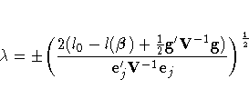
Convergence is declared on the current iteration if the following
two conditions are satisfied:
is 1E-4).
Convergence is declared on the current iteration if the following
two conditions are satisfied:


where zp is the 100pth percentile of the standard normal
distribution, ![]() is the maximum likelihood
estimate of
is the maximum likelihood
estimate of ![]() , and
, and
![]() is the standard error estimate of
is the standard error estimate of ![]() .
.
|
Chapter Contents |
Previous |
Next |
Top |
Copyright © 1999 by SAS Institute Inc., Cary, NC, USA. All rights reserved.