Chapter Contents
Previous
Next
|
Chapter Contents |
Previous |
Next |
| The LOGISTIC Procedure |
When fitting a model, there are several problems that can cause the goodness-of-fit statistics to exceed their degrees of freedom. Among these are such problems as outliers in the data, using the wrong link function, omitting important terms from the model, and needing to transform some predictors. These problems should be eliminated before proceeding to use the following methods to correct for overdispersion.
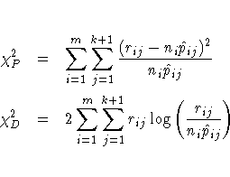
The Pearson chi-square statistic ![]() and the deviance
and the deviance ![]() are given by
are given by


In order for the Pearson statistic and the deviance to be distributed as chi-square, there must be sufficient replication within the subpopulations. When this is not true, the data are sparse, and the p-values for these statistics are not valid and should be ignored. Similarly, these statistics, divided by their degrees of freedom, cannot serve as indicators of overdispersion. A large difference between the Pearson statistic and the deviance provides some evidence that the data are too sparse to use either statistic.
You can use the AGGREGATE (or AGGREGATE=) option to define the subpopulation profiles. If you do not specify this option, each observation is regarded as coming from a separate subpopulation. For events/trials syntax, each observation represents n Bernoulli trials, where n is the value of the trials variable; for single-trial syntax, each observation represents a single trial. Without the AGGREGATE (or AGGREGATE=) option, the Pearson chi-square statistic and the deviance are calculated only for events/trials syntax.
Note that the parameter estimates are not changed by this method. However, their standard errors are adjusted for overdispersion, affecting their significance tests.

![E(r_i) = n_i p_i {and}
V(r_i) = n_i p_i (1-p_i) [1 + (n_i - 1) \phi]](images/lgseq201.gif)
Williams (1982) estimates the unknown parameter ![]() by
equating the value of Pearson's chi-square statistic for the
full model
to its approximate expected value.
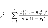
Suppose wi* is the weight
associated with the ith observation. The Pearson chi-square
statistic is given by
by
equating the value of Pearson's chi-square statistic for the
full model
to its approximate expected value.
Suppose wi* is the weight
associated with the ith observation. The Pearson chi-square
statistic is given by

![E_{\chi^2} = \sum_{i=1}^n w_i^* ( 1 - w_i^* v_i d_i)[1 + \phi (n_i - 1)]](images/lgseq203.gif)
At the start,
let wi*=1 and let pi be approximated by ri/ni, i = 1,2, ... ,n.
If you apply these weights and approximated probabilities to
![]() and
and ![]() and then equate them,
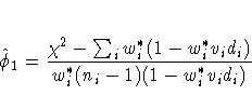
an initial estimate of
and then equate them,
an initial estimate of ![]() is
therefore
is
therefore


Once ![]() has been estimated by
has been estimated by ![]() under the full model,
weights of
under the full model,
weights of ![]() can be used in fitting models
that have fewer terms than the full model.
See Example 39.8 for an illustration.
can be used in fitting models
that have fewer terms than the full model.
See Example 39.8 for an illustration.
|
Chapter Contents |
Previous |
Next |
Top |
Copyright © 1999 by SAS Institute Inc., Cary, NC, USA. All rights reserved.