STAT 330: 95-3

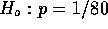
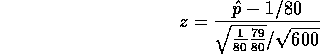
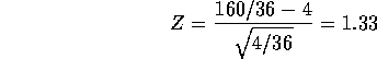
Assignment 2 Solutions

1. Let be the average reaction time for experienced swimmers. (I remark that this is probably one of the many times when the sample is not randomly drawn from some population and therefore the confidence methodology is not appropriate; what set of experienced swimmers is being talked about? If the answer is that this set of 16 is a random sample from a large group then is the average for that large group. If the answer is, as I suspect, that this is just a convenient group of 16 swimmers who happened to be available then I do not quite see what is. I will set this aside to do the arithmetic but I would be unhappy about doing this calculation for a client.) Assuming that the population of reaction times for experienced swimmers has a normal distribution then the confidence interval is

   

2. Chapter 7, Q 42 on page 302. This experiment is probably subject to the same criticism as the previous one.
   1. A good plot to look at here is a Q-Q plot in which the 16 numbers, sorted into order from smallest to largest, are plotted against the 16 z values which split the area under the normal curve into 17 equal pieces. Since 1/17 = 0.0588 the first such value is -1.565. Similarly, 2/17 = 0.118 is the area to the left of -1.18 and the second smallest value would be plotted against this.

      I did not talk about this in class so all you could really do is look for obvious outliers or asymmetry. I see no sign of any problem.

   2. I get and . The t multiplier on 15 degrees of freedom is 2.13 so the interval is .

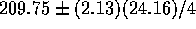3. Chapter 8, Q 60 p 343: Let be the mean soil heat flux for plots covered with coal dust. The null hypothesis is that and the alternative is (you are asked about increasing the mean flux). The sample mean is 30.7875 and leading to and % (I used a package to get P) so that the the null hypothesis is not rejected. If you had switched the role of the hypotheses you would have concluded that the the hypothesis cannot be rejected either -- the data are just not very conclusive.

4. From text: Chapter 8, Q 64 p 344 It seems obvious that the more serious error would be to assume that the average flame standard met the standard when it did not so, letting denote the average flame time for strips of this sort of nightwear, we should test 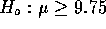against 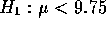. When you do the arithmetic however, the sample mean is 9.75 + ( the average of the list 10, 18, 0, 2, -8, 12, -8, 19, 10, 0, 18, 17, 24, 13, 20, 20, 18, 17, 14)/100 which comes to 9.8525. This is well over 9.75 so if you test the null I just suggested you would simply not reject it (and this would mean not permitting the use of this nightwear). On the other hand the hypothesis that results in a t statistic of 4.75 and a P value that is very small so this hypothesis is not tenable. Thus in this case the evidence is clear that the standard is not met. It is clear that the second hypothesis is the one the book expected you to test but also seems clear that the process of making the more serious error be the type I error leads to the other hypothesis, namely, being the null. The required assumption is that the population of measured flame times have a normal distribution. The point of my arithmetic short cut is that 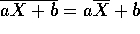and that the SD of the numbers aX+b is |a| times the SD of the X's.

5. Chapter 8, Q 66 p 344: Let p be the proportion of US penal institution inmates having the chromosome defect. The null hypothesis is and the alternative is that . The relevant test statistic is

   

   where 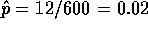. Thus , and the test rejects at the 20% level but not at the 5% level. In part a) the type of error you might be making is type II, incorrectly accepting the null (because you do accept the null in a).

6. Chapter 8, Q 70 p 344: I think the word ``suggest'' means offer evidence for the assertion that . But hypothesis testing measures against an assertion so you have to make the assertion you want evidence for the alternative and thus the assertion you want evidence against the null. Thus we get or and . The resulting test statistic is

   

   which leads to a P-value of 9.18% which I would describe as some, weak, evidence against the null hypothesis and in favour of the assertion that .

7. Chapter 7, Q 45:
   1. You are asked to compute where , and 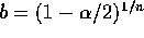. The definition of density means that this is

      

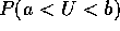
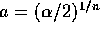
      Now solve to get and similarly for a.

   2. If then and if then . The probability of this event is just as in a) but with the limits a and b changed to and 1 so the probability is and the interval runs from Y to .

   3. The length of the two intervals is Y times which is shorter in the case of b) (For instance in the example with and n = 5 we find the interval in a) has length 4.56 while that in b has length 3.45.) For the data in hand , and the limits in b) are 4.2 to 7.65.

      I remark that this model assumes that the buses always run exactly minutes apart and the writer arrives at a ``random time'' --- not very realistic.

• About this document ...