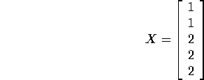
- Assume that the individual lengths satisfy, for i from 1 to 2 and
j from 1 to 2 (for i=1) or 1 to 3 (for i=2),

where the errors
 are independent normal variables
and have mean 0 and
variance
  . What is the design matrix for this linear model? [2 marks]
Solution:

- Give an explicit, simple, formula for the least squares estimate
of
 ; I do not want a general formula such as
  .
[4 marks]
Solution:

and

so that

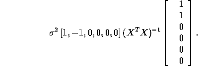
- Give the mean and variance of the estimator in (b). [2 marks]
Solution:

and

- The average measurements
 also satisfy a linear model

- What is
 in terms of
  ?
[1 marks]
Solution:

- What is the joint distribution of
 ?
In particular what are the variances and means of each
  ?
[3 marks]
Solution:

so that
 has a multivariate normal distribution
with mean 0 and variance covariance matrix

- What is the design matrix of this linear model?
[1 marks]
Solution:

- What is
- Show that the weighted least squares estimate of
 is
is

[4 marks]
Solution: The variances of the errors are
 and
and  so that
the weights are
  and
and  . Then

and

so that

- What is the distribution of
 . [2 marks]
Solution: Normal with mean
 and variance
  .
. - Why would analysis of the original variables
 be better
than analysis of the
  ? [1 mark]
Solution: We would have 4 degrees of freedom for error rather than 1.
| Vars | ESS | Vars | ESS | Vars | ESS | Vars | ESS |
|
| 154 | | 109 | | 133 | | 139 |
|
| 156 | | 144 | | 175 | | 132 |
|
| 203 | | 146 | | 106 | All | 104 |
|
| 250 | | 150 | | 107 | None | 506 |
- Does adding the variables
 and
and  to the model containing
 and
and  significantly improve the fit? [6 marks]
Solution: This compares the model with all variables in to the model with just
 and
and  and
so

This is much less than 1 so the added variables are not significant.
- Use Backwards selection with a 10% significance level to stay
to select a suitable subset of regression variables. [8 marks]
Solution: We begin with all variables. Among the 3 variable models the model containing only
 ,
,  and
and  has the smallest error sum of squares
so if we delete a variable it must be
  . The F statistic is

so we delete
 . Among the two variable models which contain 2 of the variables
 ,
,  and
and  the model containing
  and
and  has the smallest
error sum of squares so we try to delete
  getting

which is still far from significant. We delete
 and look at 1 variable
models which either use
  or
or  . The smallest error SS is for
  so we
try to delete
  getting

We compare this to the F tables with 1 numerator and 17 denominator degrees of freedom and see that
 so that
  and
and  will be retained.
 - If the estimated slope associated with
 in the model including
  and
and  only as predictors
is positive what is the value of the t statistics for testing
the hypothesis that the true coefficient of
  is 0? [1 mark]
Solution:
 .
.
Model I
![]()
the error sum of squares is 85355 and the estimates are
|
| |
| 37.26 | 0.65 |
Model II
![]()
the error sum of squares is 66115 and the estimates are
|
| | | | | |
| 14.2424 | 67.5325 | 48.3918 | 49.6033 | 68.7786 | 0.5509 |

Model III
![]()
the error sum of squares is 62433 and the estimates are
|
| | | | | |
| 52.04954 | -68.05918 | 62.48453 | 46.66416 | 112.529 | |
|
| | | | | |
| 0.2309892 | 1.619385 | 0.4313726 | 0.5757114 | 0.1818949 |
- Of the three models, based on the information available to you,
which model provides the best fit to the data. [10 marks]
Solution: Testing Model III vs Model II we get

which is not significant. Thus Model II is preferred to Model III. Comparing Model II to Model I we have

which leads to a P-value around 0.03 so that Model II is preferred to Model I.
- There are 10 possible comparisons between pairs of treatments. It is desired to
give simultaneous 95% confidence intervals for all possible comparisons based
based on the second model above. I want you to show clearly that you know how to get these
ten confidence intervals. Your answer will include a clear description of the parameters
for which intervals are needed, written in terms of the notation used above for the second
model and the resulting confidence interval for the difference between treatment A
and treatment B with all the numbers filled in. You need not work it out to the point of
a numerical value for the lower and upper limit. [5 marks]
Solution: I want confidence intervals for the 10 values of
 with i;SPMlt;j. To get
simultaneous 95% confidence intervals you divide
  by 10 and just work
out ordinary 99.5% confidence intervals. The t multiplier is around 2.96. z
You also need a standard error for
  which is
the square root of

You estimate
 using 66115/44 and get

- Examine the residual plots attached for the three models.
Is there anything wrong with our fit?
If so suggest what you might try next. Be quite clear. [5 marks]
Solution: The plots show clear signs of heteroscedasticity; a transformation might be useful. (In fact taking logs is the thing to do.)
- I attach a table of regression diagnostics for the fit to model II above.
For each diagnostic review the values and comment on whether or not they show
any problems and which cases might warrant further examination. [5 marks]
Solution:
I just wanted people to compare the various statistics to the guidelines in the text. For the externally studentized residuals I was looking for some mention of the Bonferroni adjustment. Cases 15 and 44 stand out as worth looking at again.