

STAT 350: Lecture 1 Example
Thermoluminescence Dating
Thermoluminescence (TL) dating can be used to determine how
old a piece of pottery is or how old a sand dune is. When
a piece of pottery is found by an archaeologist it is ground
up and split into small samples. The samples are irradiated with
different amounts of gamma radiation and then heated in an oven.
At temperatures around 300 Celsius they glow with blue light called
thermoluminescence. The amount of light given off, Y depends on
the dose D of radiation given by the analyst
(and also on the amount of radiation
--cosmic rays or radiation from trace isotopes in the ground--
to which the pot or sand was exposed while buried).
Several models are in use:
- a straight-line model,

- a quadratic model,

- a cubic model,

- and a saturating exponential model,

Of these the first three are linear models while the fourth is not. In the
first three cases the mean  can be differentiated with respect to
any
can be differentiated with respect to
any  and you get a known (measured) constant.
Thus for example in the second model
and you get a known (measured) constant.
Thus for example in the second model

For the last model, however, the derivatives depend on unknown parameters, such
as,
which is not known since it involves  and
and  .
.
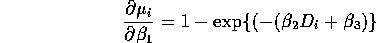
Here is a plot of the data with the least squares line drawn in.
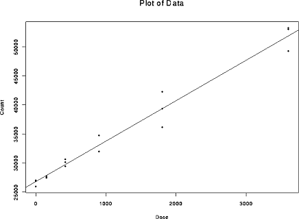 And here is the same plot with the least squares fit of the quadratic model.
 You will see that the two fits are virtually indistinguishable.
In this course we will want to test the hypothesis that the
term in the quadratic model can be left out. To see the importance of this
consider the use to which these models are put. Physicists reckon that the
intercept term
You will see that the two fits are virtually indistinguishable.
In this course we will want to test the hypothesis that the
term in the quadratic model can be left out. To see the importance of this
consider the use to which these models are put. Physicists reckon that the
intercept term  which is the amount of TL if you don't add
any radiation is the TL due to the exposure to cosmic rays and so on
while buried. The total exposure while buried is equivalent to some
dose
which is the amount of TL if you don't add
any radiation is the TL due to the exposure to cosmic rays and so on
while buried. The total exposure while buried is equivalent to some
dose  of added radiation called the ``equivalent dose'',
equivalent in the sense that
of added radiation called the ``equivalent dose'',
equivalent in the sense that  if a
straightline model is appropriate. This dose is measured by finding the value
of D which would produce a predicted TL equal to 0, that is,
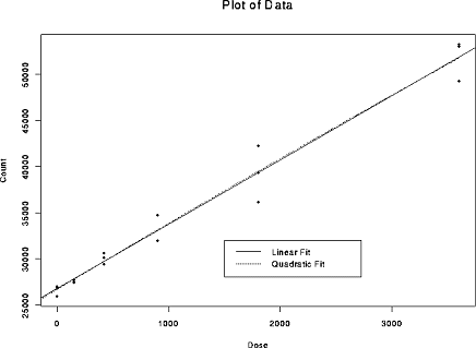
by extending the graph to negative doses until the fit crosses the x axis.
In the next plot
if a
straightline model is appropriate. This dose is measured by finding the value
of D which would produce a predicted TL equal to 0, that is,
by extending the graph to negative doses until the fit crosses the x axis.
In the next plot
 you can see that the linear and quadratic fits do cross the x axis (or y=0)
at different places.
you can see that the linear and quadratic fits do cross the x axis (or y=0)
at different places.
We will be fitting linear models (and near the end of the course non-linear models
like the saturating exponential) by least squares. We will examine residual plots:
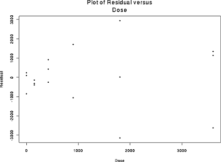 to judge whether or not the model assumptions are adequate. In this case the plot
shows clear signs of heteroscedasticity -- unequal variances.
We will look at Q-Q plots of the residuals to judge normality.
to judge whether or not the model assumptions are adequate. In this case the plot
shows clear signs of heteroscedasticity -- unequal variances.
We will look at Q-Q plots of the residuals to judge normality.
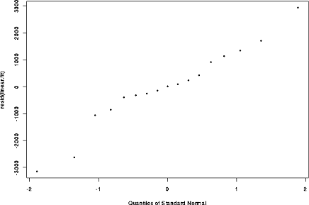 The plot is not straight and so the assumption of normally distributed
errors would also be in doubt; this problem is probably irrelevant in
view of the heteroscedasticity, however.
The plot is not straight and so the assumption of normally distributed
errors would also be in doubt; this problem is probably irrelevant in
view of the heteroscedasticity, however.
Richard Lockhart
Mon Mar 3 13:25:44 PST 1997