STAT 350: Lecture 4 Example

The sum of squares decomposition in one example

See Lecture 2 for more about this example. There I showed the design matrix for the model

with .

The data consist of blood coagulation times for 24 animals fed one of 4 different diets. In the following I write the data in a table and decompose the table into a sum of several tables. The 4 columns of the table correspond to Diets A, B, C and D. You should think of the entries in each table as being stacked up into a column vector, but the tables save space.

The design matrix can be partitioned into a column of 1s and 3 other columns. You should compute the product and get

The matrix is just

The matrix can be inverted using a program like Maple. I found that

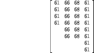
It now takes quite a bit of algebra to verify that the vector of fitted values can be computed by simply averaging the data in each column. That is, the fitted value, is the table

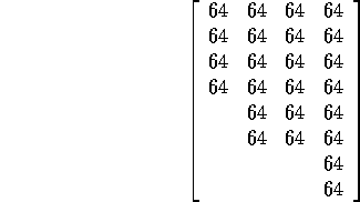
On the other hand fitting the model with a design matrix consisting only of a column of 1s just leads to (notation from the lecture) given by

Now in class I gave the decomposition

which corresponds to the following identity:

The sums of squares of the entries of each of these arrays are as follows. On the left hand side . This is the uncorrected total sum of squares. The first term on the right hand side gives . This term is sometimes put in ANOVA tables as the Sum of Squares due to the Grand Mean but it is usually subtracted from the total to produce the Total Sum of Squares we usually put at the bottom of the table and often called the Corrected (or Adjusted) Total Sum of Squares. In this case the corrected sum of squares is the squared length of the table

which is 340.

The second term on the right hand side of the equation has squared length (which is the Treatment Sum of Squares produced by SAS). The formula for this Sum of Squares is

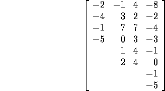
but I want you to see that the formula is just the squared length of the vector of individual sample means minus the grand mean. The last vector of the decomposition is called the residual vector and has squared length . Corresponding to the decomposition of the total squared length of the data vector is a decomposition of its dimension, 24, into the dimensions of subspaces. For instance the grand mean is always a multiple of the single vector all of whose entries are 1; this describes a one dimensional space (this is just another way of saying that the reduced is in the column space of the reduced model design matrix). The second vector, of deviations from a grand mean lies in the three dimensional subspace of tables which are constant in each column and have a total equal to 0. Similarly the vector of residuals lies in a 20 dimensional subspace - the set of all tables whose columns sum to 0. This decomposition of dimensions is the decomposition fo degrees of freedom. So 24 = 1+3+20 and the degrees of freedom for treatment and error are 3 and 20 respectively. The vector whose squared length is the Corrected Total Sum of Squares lies in the 23 dimensional subspace of vectors whose entries sum to 1; this produces the 23 total degrees of freedom in the usual ANOVA table.