STAT 350: 95-3

Assignment 4

Part A

From text page 254-255, 6.15 c, d, e, f, g, 6.16, 6.17. Page 257 6.25 and 6.26. Page 324 7.46. Page 394 9.11. Page 398 9.25.

6.15-17 I began with this SAS code:

  data patsat;
  infile '615.dat' firstobs=2;
  input Satisf Age Severity Anxiety ;
  proc glm  data=patsat;
   model Satisf = Age Severity Anxiety ;
   estimate '617a' Intercept 1 Age 35 Severity 45 Anxiety 2.2;
   output out=anovres r=resid p=fitted;
  proc print data=anovres;

This code produces the anova table, t tests for individual coefficients and the estimates required for predicted values; it also prints out residuals for use later. The output shows:

6.15 c The fitted regression function is

The question asks for an interpretation of . Mathematically it means that holding Age and Anxiety constant an increase of 1 unit in severity of disease is associated with an average decrease of 0.666 units in Satisfaction. The book wants you, however, to think about the real world interpretation. Patients with more severe illnesses are less satisfied with the hospital, after adjusting for Age and Anxiety level. Whether the amount less is a lot or a little depends on the units in which severity and satisfaction are measured and since these are indices we cannot really tell.

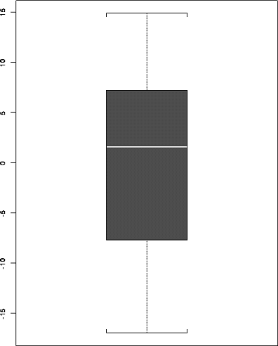
6.15 d Here is a box plot of the (raw) residuals from Splus; I see no problem with outliers.

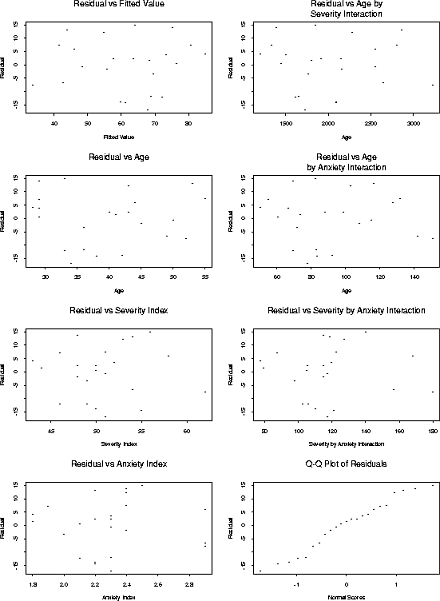
6.15 e Here is a set of plots from Splus

There seems to be no particular problem in any of the 7 plots. The plots show no need for inclusion of the interactions terms and no sign of non-normality.

6.15 f You need replicate observations to compute a pure error sum of squares and you don't have any such. Sometimes people try a clustering technique to split the data set into groups of `near replicates' and then treating these groups as groups of replicates but the technique doesn't work all that well.

6.15 g You have to look in the text for this one. The test regresses squared residuals on the covariates and computes a statistic which looks a lot like an F test (because it was intended to be analogous to such an F test) except for the numerator not being divided by degrees of freedom and the denominator being somewhat different; see page 115 and page 239. I used the code above to print out a data set which includes the needed residuals. I saved the results in a file, deleting all the extra output, and then ran this SAS code:

 options pagesize=60 linesize=80;
 data patsatr;
  infile '615res.dat' firstobs=2;
  input Obs Satisf Age Severity Anxiety Resid Fitted;
  rsq=Resid**2;
 proc glm  data=patsatr;
   model rsq = Age Severity Anxiety ;
 run;

You take the Model Sum of Squares from the output which is 24518 and the Error Sum of Squares from the original output which is 2011.6 and compute

From table B 3 we see the P-value is between 0.1 and 0.9 (Splus gives a P value of 0.65) so that there is no evidence of heteroscedasticity related to the values of the covariates.

6.16 a The overall F statistic is 13.01 with a P-value of 0.0001 so the hypothesis that is rejected at the level 0.1 and, indeed, at any level down to 0.0001. The test implies that at least one of the three coefficients is not 0.

6.16 b The text intended a joint interval using the Bonferroni procedure: estimate plus or minus times estimated standard errors. The estimates and estimated standard errors are in the SAS output

                            T for H0:    Pr > |T|   Std Error of
Parameter      Estimate    Parameter=0                Estimate
INTERCEPT   162.8758987           6.32     0.0001    25.77565190
AGE          -1.2103182          -4.01     0.0007     0.30145159
SEVERITY     -0.6659056          -0.81     0.4274     0.82099695
ANXIETY      -8.6130315          -0.70     0.4902    12.24125126

The required t critical value is 2.29; you would need to interpolate in the tables page 1337 between 0.98 and 0.985 since the lower tail area you actually want is 1-0.05/3=0.98333. Go 2/3 of the way from 2.205 to 2.346. I actually used Splus.

6.16 c From the output the value of is 0.67. We sometimes describe this as meaning that 2/3 of the variance in patient satisfaction is accounted for by these three covariates. This is a fairly high but not wonderful multiple correlation.

6.17 a The output of the estimate statement is

                            T for H0:    Pr > |T|   Std Error of
Parameter      Estimate    Parameter=0                Estimate
617a         71.6003409          16.11     0.0001     4.44322423

so that the estimate is . If you want to predict an individual observation, though, as in b) you have to take a standard error of the form . Notice that the prediction interval is much wider. For a new individual with covariate values 35, 45 and 2.2, there is roughly a 90% chance that the satisfaction level will be in the range .

9.11 SAS CODE

options pagesize=60 linesize=80;
data patsat;
 infile '615.dat' firstobs=2;
 input Satisf Age Severity Anxiety ;
proc reg  data=patsat;
 model Satisf = Age Severity Anxiety /XPX I;
 output out=anovres r=resid p=fitted 
    h=hat dffits=dffits cookd=cookd  
    rstudent=rstudent press=press;
proc print data=anovres;

The output shows that

9.11 a The largest externally studentized residual is for observation 14 at -1.81. This should be compared to the value roughly. (I used the 0.9975 column; you really want 0.9978 so my critical point is a bit too small.) There are no surprising Y outliers.

9.11 b The largest leverage is 0.34 (for observation 9) which should, according to the text (p 377) be compared to 2(4)/23=.35 or so. This is not too large for such a small data set but it would probably warrant a quick look at this point and at case 15 whose leverage is 0.31.

9.11 c You are supposed to compute when . I printed out the entries in (using the I option on the model statement. I used S to compute the desired leverage, getting 0.87 which is an unusually large leverage; I conclude that this would be a substantial extrapolation.

9.11 d The relevant lines of output are

            S                                                   R
            E  A                                                S
      S     V  N     F                                          T        D
      A     E  X     I        R       C                P        U        F
      T     R  I     T        E       O                R        D        F
   O  I  A  I  E     T        S       O       H        E        E        I
   B  S  G  T  T     E        I       K       A        S        N        T
   S  F  E  Y  Y     D        D       D       T        S        T        S

  14 51 34 51 2.3 67.9539 -16.9539 0.05661 0.07185 -18.2663 -1.80980 -0.50353

The values of DFFITS and COOKD are not too large; see Lecture 21 for guidelines. I conclude this data point is ok.

9.11 e I did this partly in S. You need to compute all the fitted values with case 14 removed; the easiest way is to delete case 14 from the data file and rerun. You get the predicted value for case 14 by subtracting the PRESS residual for case 14 from the true Y for case 14. I got

which seems pretty minor.

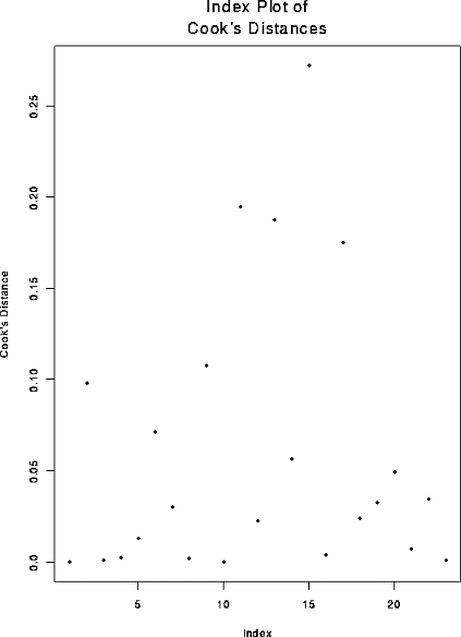
9.11 f You are to plot against i. The result is

Case 15 looks a bit surprising and should probably be investigated.

6.25 You are to choose the s to minimize

which simply is ordinary least squares with response variable

and 3 parameters to be adjusted. In SAS you would create a variable having and regress it on and .

6.26 The multiple correlation coefficient is

Now and . If we regress on then the correlation coefficient is

Squaring r we see that we should prove

In lecture 4 or so I showed you that the Regression Sum of Squares is

Now

The first term is 0 because the vector of residuals is orthogonal to the fitted vector. The last term is 0 because the sum of the residuals is 0 in any model with an intercept. In the middle term because . Hence

and this finishes the problem.

7.46 The reduced models are

a)



b)



c)



d)

9.25 If X is invertible then so that

The diagonal elements of the identity matrix are all 1 and so that .

Part B

1. In assignment 2 in question 2 you dealt with variables . In class I stated that the if the covariance between two components of a multivariate normal vector is 0 then the components are independent, but I indicated a proof only when the multivariate normal distribution in question has a density. In this case the variance matrix is singular so there is no density. However, in terms of the original Z it is possible to find two independent functions of Z such that are a function of the first function while is a function of the second.
   1. Let , and . Show that has a multivariate normal distribution and identify the mean and variance of U.

      Solution: We have U=AZ where the matrix A is

      

      Thus U has a multivariate normal distribution with mean A0=0 and variance which may be multiplied out to give

      

   2. Use the result in class, for multivariate normals which have a density to show that is independent of .

      Solution: The variance covariance matrix in the previous part is block diagonal with a 2 by 2 block and a 1 by 1 block, so the first two components are independent of the last component.

   3. Express as a function of U.

      Solution: . Now so

      

      and

      

   4. Use the fact that if and are independent then so are and for any functions G and H to show that is independent of .

      Solution: The function G is

      

      while

      

      Since is independent of we see is independent of .

   5. Express the sample variance of the in terms of U and use this to show that has a distribution on 2 degrees of freedom.

      Solution: This question is wrong! You can write

      

      as

      

      but this is not a straightforward sum of two squares of standard normals as written. The trick to do the real question is two write the numerator in the sample variance for a sample of 3 as the sum of the numerator for the sample variance of the sample of size 2 plus another term. These two terms turn out to be independent variables except for a factor of .

2. In class I discussed the general formula for a multivariate normal density. Suppose that and are independent standard normal variables. Assume that and . Find the joint density of and by evaluating the formulas I gave in class. Express as a double integral. I want to see the integrand and the limits of integration but you need not try to do the integral.

   Solution: The density in class was

   

   where .

   The entries in are c and f and we have

   

   Then

   

   and

   

   Putting together all the algebra gives

   

   where the exponent is the quadratic function

   

   To compute we take the joint density of and and integrate it over the set of such that to get