STAT 380: Introduction to Stochastic Processes

Course outline:

Today's lecture Summary
Some Basic Examples

Example 1: Three cards: one red on both sides, one black on both sides, one black on one side, red on the other. Shuffle, pick card at random. Side up is Black. What is the probability the side down is Black?

Solution: To do this carefully, enumerate sample space, $\Omega$, of all possible outcomes. Six sides to the three cards. Label three red sides 1, 2, 3 with sides 1, 2 on the all red card (card # 1). Label three black sides 4, 5, 6 with 3, 4 on opposite sides of mixed card (card #2). Define some events:
\begin{align*}A_i & = \{\text{side $i$\space shows face up}\}
\\
B & = \{\text{...
...showing is black}\}
\\
C_j & = \{\text{card $j$\space is chosen}\}
\end{align*}

One representation $\Omega=\{1,2,3,4,5,6\}$. Then $A_i = \{i\}$, $B=\{4,5,6\}$, $C_1=\{1,2\}$ and so on.

Modelling: assumptions about some probabilities; deduce probabilities of other events. In example simplest model is

All of the Ai are equally likely.

Apply two rules:

\begin{displaymath}P(\cup_1^6 A_i) = \sum_1^6 P(A_i) \quad\text{and} \quad
P(\Omega) = 1
\end{displaymath}

to get, for $i=1,\ldots,6$,

\begin{displaymath}P(A_i) = \frac{1}{6}
\end{displaymath}

Question was about down side of card. We have been told B has happened. Event that a black side is down is $D=\{3,5,6\}$. (Of course B has happened rules out 3.)

Definition of conditional probability:

\begin{displaymath}P(D\vert B) = \frac{P(D\cap B)}{P(B)} = \frac{P(\{5,6\})}{P(\{4,5,6\})} =
\frac{2}{3}
\end{displaymath}

Example 2: Monte Hall, Let's Make a Deal. Monte shows you 3 doors. Prize hidden behind one. You pick a door. Monte opens a door you didn't pick; shows you no prize; offers to let you switch to the third door. Do you switch?

Sample space: typical element is (a,b,c) where a is number of door with prize, b is number of your first pick and c is door Monte opens with no prize.

(1,1,2) (1,1,3) (1,2,3) (1,3,2)
(2,1,3) (2,2,1) (2,2,3) (2,3,1)
(3,1,2) (3,2,1) (3,3,1) (3,3,2)

Model? Traditionally we define events like
\begin{align*}A_i & = \{\text{Prize behind door $i$ }\}
\\
B_j & = \{\text{You choose door $j$ }\}
\end{align*}
and assume that each Ai has chance 1/3. We are assuming we have no prior reason to suppose Monte favours one door. But these and all other probabilities depend on the behaviour of people so are open to discussion.

The event LS, that you lose if you switch is
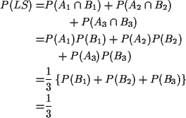
\begin{displaymath}(A_1\cap B_1) \cup (A_2\cap B_2) \cup (A_3\cap B_3)
\end{displaymath}

The natural modelling assumption, which captures the idea that you have no idea where the prize is hidden, is that each Aiis independent of each Bj, that is,

\begin{displaymath}P(A_i \cap B_j) = P(A_i)P(B_j)
\end{displaymath}

Usually we would phrase this assumption in terms of two random variables, M, the door with the prize, and C the door you choose. We are assuming that M and C are independent. Then
\begin{align*}P(LS) = & P(A_1\cap B_1) + P(A_2\cap B_2)
\\
& \qquad + P(A_3\ca...
...rac{1}{3}\left\{P(B_1) + P(B_2) +P(B_3)\right\}
\\
= &\frac{1}{3}
\end{align*}

So the event you win by switching has probability 2/3 and you should switch.

Usual phrasing of problem. You pick 1, Monte shows 3. Should you take 2? Let S be rv S = door Monte shows you. Question:

P(M=1|C=1, S=3)

Modelling assumptions do not determine this; it depends on Monte's method for choosing door to show when he has a choice. Two simple cases:

1.
Monte picks at random so

P(S=3|M=1,C=1) = 1/2

2.
Monte chooses the door with the largest possible number:

P(S=3|M=1,C=1) = 1

Use Bayes' rule:
\begin{multline*}P(M=1\vert C=1, S=3)
\\
= \frac{P(M=1,C=1, S=3)}{P(C=1,S=3)}
\end{multline*}
Numerator is
\begin{multline*}P(S=3\vert M=1,C=1) P(M=1,C=1)
\\
= P(S=3\vert M=1,C=1)P(C=1)/3
\end{multline*}
Denominator is
\begin{multline*}P(S=3\vert M=1,C=1) P(M=1,C=1)
\\
+
P(S=3\vert M=2,C=1) P(M=2,C=1)
\\
+P(S=3\vert M=3,C=1) P(M=3,C=1)
\end{multline*}
which simplifies to
\begin{multline*}P(S=3\vert M=1,C=1)P(M=1)P(C=1)
\\
+1 \cdot P(M=2)P(C=1)
\\
+0 \cdot P(M=3)P(C=1)
\end{multline*}
which in turn is

\begin{displaymath}\left\{P(S=3\vert M=1,C=1)+1\right\}P(C=1)/3
\end{displaymath}

For case 1 we get

\begin{displaymath}P(M=1\vert C=1, S=3) = \frac{1/2}{1/2 + 1} = \frac{1}{3}
\end{displaymath}

while for case 2 we get

\begin{displaymath}P(M=1\vert C=1, S=3) = \frac{1}{1+1} =\frac{1}{2}
\end{displaymath}

Notice that in case 2 if we pick door 1 and Monte shows us door 2 we should definitely switch. Notice also that it would be normal to assume that Monte used the case 1 algorithm to pick the door to show when he has a choice; otherwise he is giving the contestant information. If the contestant knows Monte is using algorithm 2 then by switching if door 2 is shown and not if door 3 is shown he wins 2/3 of the time which is as good as the always switch strategy.

Example 3: Survival of family names. Traditionally: family name follows sons. Given man at end of 20th century. Probability descendant (male) with same last name alive at end of 21st century? or end of 30th century?

Simplified model: count generations not years. Compute probability, of survival of name for n generations.

Technically easier to compute qn, probability of extinction by generation n.

Useful rvs:

\begin{displaymath}X= \text{\char93  of male children of first man}
\end{displaymath}


\begin{displaymath}Z_k = \text{\char93  of male children in generation $k$}
\end{displaymath}

Event of interest:

\begin{displaymath}E_n = \{ Z_n=0\}
\end{displaymath}

Break up En:

\begin{displaymath}q_n=P(E_n) = \sum_{k=0}^\infty P(E_n\cap \{ X=k\})
\end{displaymath}

Now look at the event $E_n\cap \{ X=k\}$. Let
\begin{align*}B_{j,n-1} =& \{ X=k\}\cap \{\text{child $j$ s line extinct}
\\
& \quad \text{ in $n-1$\space generations}\}
\end{align*}
Then

\begin{displaymath}E_n\cap \{ X=k\} =\cap_{j=1}^k B_{j,n-1}
\end{displaymath}

Now add modelling assumptions:
1.
Given (conditional on) X=k the events Bj,n-1 are independent. In other words: one son's descendants don't affect other sons' descendants.

2.
Given X=k the probability of Bj,n-1 is qn-1. In other words: sons are just like the parent.

Now add notation P(X=k) = pk.
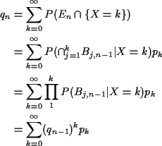
\begin{align*}q_n & = \sum_{k=0}^\infty P(E_n\cap \{ X=k\})
\\
& = \sum_{k=0}^\...
...P(B_{j,n-1}\vert X=k) p_k
\\
& = \sum_{k=0}^\infty (q_{n-1})^k p_k
\end{align*}
Probability generating function:

\begin{displaymath}\phi(s) = \sum_{k=0}^\infty s^k p_k = {\rm E}(s^X)
\end{displaymath}

We have found

q1 = p0

and

\begin{displaymath}q_n = \phi(q_{n-1})
\end{displaymath}

Notice that $q_1 \ge q_2 \ge \cdots$ so that the limit of the qn, say $q_\infty$, must exist and (because $\phi$ is continuous) solve

\begin{displaymath}q_\infty = \phi(q_\infty)
\end{displaymath}

Special cases

Geometric Distribution: Assume

\begin{displaymath}P(X=k) = (1-\theta)^k \theta \qquad k=0,1,2,\ldots
\end{displaymath}

(X is number of failures before first success. Trials are Bernoulli; $\theta$ is probability of success.)

Then
\begin{align*}\phi(s) & = \sum_0^\infty s^k (1-\theta)^k \theta
\\
& = \theta \...
...fty \left[s(1-\theta)\right]^k
\\
& = \frac{\theta}{1-s(1-\theta)}
\end{align*}
Set $\phi(s) = s$ to get

\begin{displaymath}s[1-s(1-\theta)]=\theta
\end{displaymath}

Two roots are

\begin{displaymath}\frac{1 \pm \sqrt{1-4\theta(1-\theta)}}{2(1-\theta)} =
\frac{1 \pm (1-2\theta)}{2(1-\theta)}
\end{displaymath}

One of the roots is 1; the other is

\begin{displaymath}\frac{\theta}{1-\theta}
\end{displaymath}

If $\theta \ge 1/2$ the only root which is a probability is 1 and $q_\infty=1$. If $\theta < 1/2$ then in fact $q_n \to q_\infty = \theta/(1-\theta)$.

Binomial($m,\theta$): If

\begin{displaymath}P(X=k) = \binom{m}{k} \theta^k(1-\theta)^{m-k} \quad k=0,\ldots, m
\end{displaymath}

then
\begin{align*}\phi(s) & = \sum_0^m \binom{m}{k} (s\theta)^k(1-\theta)^{m-k}
\\
& = (1-\theta+s\theta)^m
\end{align*}
The equation $\phi(s) = s$ has two roots. One is 1. The other is less than 1 if and only if $mp={\rm E}(X) > 1$.

Poisson($\lambda$): Now

\begin{displaymath}P(X=k) = e^{-\lambda} \lambda^k/k! \quad k=0,1,\ldots
\end{displaymath}

and

\begin{displaymath}\phi(s) = e^{\lambda(s-1)}
\end{displaymath}

The equation $\phi(s) = s$ has two roots. One is 1. The other is less than 1 if and only if $\lambda = {\rm E}(X) > 1$.

Important Points:

Example 3: Mean values

Zn = total number of sons in generation n.

Z0=1 for convenience.

Compute ${\rm E}(Z_n)$.

Recall definition of expected value:

If X is discrete then

\begin{displaymath}{\rm E}(X) = \sum_x x P(X=x)
\end{displaymath}

If X is absolutely continuous then

\begin{displaymath}{\rm E}(X) = \int_{-\infty}^\infty x f(x) dx
\end{displaymath}

Theorem: If Y=g(X), X has density f then

\begin{displaymath}{\rm E}(Y) = {\rm E}(g(X)) =\int g(x) f(x) dx
\end{displaymath}

Key properties of ${\rm E}$:

1: If $X\ge 0$ then ${\rm E}(X) \ge 0$. Equals iff P(X=0)=1.

2: ${\rm E}(aX+bY) = a{\rm E}(X) +b{\rm E}(Y)$.

3: If $0 \le X_1 \le X_2 \le \cdots$ then

\begin{displaymath}{\rm E}(\lim X_n) = \lim {\rm E}(X_n)
\end{displaymath}

4: ${\rm E}(1) = 1$.

Conditional Expectations

If X, Y, two discrete random variables then

\begin{displaymath}{\rm E}(Y\vert X=x) = \sum_y y P(Y=y\vert X=x)
\end{displaymath}

Extension to absolutely continuous case:

Joint pmf of X and Y is defined as

p(x,y) = P(X=x,Y=y)

Notice: The pmf of X is

\begin{displaymath}p_X(x) = \sum_y p(x,y)
\end{displaymath}

Analogue for densities: joint density of X,Y is

\begin{displaymath}f(x,y) dx dy \approx P(x \le X \le X+dx, y \le Y \le y+dy)
\end{displaymath}

Interpretation is that

\begin{displaymath}P(X \in A, Y \in B) = \int_A \int_B f(x,y) dy dx
\end{displaymath}

Property: if X,Y have joint density f(x,y) then X has density

\begin{displaymath}f_X(x) = \int_y f(x,y) dy
\end{displaymath}

Sums for discrete rvs are replaced by integrals.

Example:

\begin{displaymath}f(x,y) = \begin{cases}x+y & 0 \le x,y \le 1
\\
0 & \text{otherwise}
\end{cases}\end{displaymath}

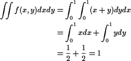
is a density because
\begin{align*}\iint f(x,y)dx dy & = \int_0^1\int_0^1 (x+y) dy dx
\\
& = \int_0^1 x dx + \int_0^1 y dy
\\
& = \frac{1}{2} + \frac{1}{2} = 1
\end{align*}

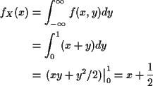
The marginal density of X is, for $0 \le x \le 1$.
\begin{align*}f_X(x) & = \int_{-\infty}^\infty f(x,y)dy
\\
& = \int_0^1 (x+y) dy
\\
& = \left.(xy+y^2/2)\right\vert _0^1
= x+\frac{1}{2}
\end{align*}

For x not in [0,1] the integral is 0 so

\begin{displaymath}f_X(x) = \begin{cases}x+\frac{1}{2} & 0 \le x \le 1
\\
0 & \text{otherwise}
\end{cases}\end{displaymath}

Conditional Densities

If X and Y have joint density fX,Y(x,y) then we define the conditional density of Y given X=x by analogy with our interpretation of densities. We take limits:
\begin{multline*}f_{Y\vert X}(y\vert x)dy \\
\approx \frac{ P(x \le X \le X+dx, y \le Y \le y+dy)}{P(x
\le X \le X+dx)}
\end{multline*}
in the sense that if we divide through by dy and let dx and dy tend to 0 the conditional density is the limit

\begin{displaymath}\frac{\lim_{dx, dy \to 0} \frac{ P(x \le X \le
X+dx, y \le Y ...
...y)}{(dx\,dy)}}{
\lim_{dx\to 0} \frac{P(x \le X \le X+dx)}{dx}}
\end{displaymath}

Going back to our interpretation of joint densities and ordinary densities we see that our definition is just

\begin{displaymath}f_{Y\vert X}(y\vert x)dy = \frac{f_{X,Y}(x,y)}{f_X(x)}
\end{displaymath}

When talking about a pair X and Y of random variables we refer to fX,Y as the joint density and to fX as the marginal density of X.

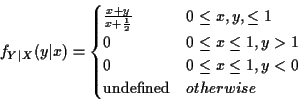
Example: For f of previous example conditional density of Y given X=x defined only for $0 \le x \le 1$:

\begin{displaymath}f_{Y\vert X}(y\vert x) = \begin{cases}
\frac{x+y}{x+\frac{1}{...
...\le x \le 1, y < 0
\\
\text{undefined} & otherwise
\end{cases}\end{displaymath}

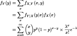
Example: X a Poisson$(\lambda)$ random variable. Observe X then toss a coin X times. Y is number of heads. P(H) = p
\begin{align*}f_Y(y) & = \sum_x f_{X,Y}(x,y)
\\
& = \sum_x f_{Y\vert X}(y\vert ...
...binom{x}{y} p^y(1-p)^{x-y} \times
\frac{\lambda^x}{x!} e^{-\lambda}
\end{align*}

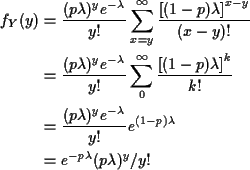
WARNING: in sum $0 \le y \le x$ is required and x, y integers so sum really runs from y to $\infty$
\begin{align*}f_Y(y) &= \frac{(p\lambda)^ye^{-\lambda}}{y!} \sum_{x=y}^\infty
\...
...\lambda}}{y!}e^{(1-p)\lambda}
\\
& = e^{-p\lambda} (p\lambda)^y/y!
\end{align*}
which is a Poisson($p\lambda$) distribution.

Conditional Expectations

If X and Y are continuous random variables with joint density fX,Y we define:

\begin{displaymath}E(Y\vert X=x) = \int y f_{Y\vert X}(y\vert x) dy
\end{displaymath}

Key properties of conditional expectation

1: If $Y\ge 0$ then ${\rm E}(Y\vert X=x) \ge 0$. Equals iff P(Y=0|X=x)=1.

2: ${\rm E}(A(X)Y+B(X)Z\vert X=x) = A(x){\rm E}(Y\vert X=x) +B(x){\rm E}(Z\vert X=x)$.

3: If Y and X are independent then

\begin{displaymath}{\rm E}(Y\vert X=x) = {\rm E}(Y)
\end{displaymath}

4: ${\rm E}(1\vert X=x) = 1$.

Example:

\begin{displaymath}f(x,y) = \begin{cases}x+y & 0 \le x,y \le 1
\\
0 & \text{otherwise}
\end{cases}\end{displaymath}

has conditional of Y|X:

\begin{displaymath}f_{Y\vert X}(y\vert x) = \begin{cases}
\frac{x+y}{x+\frac{1}{...
...\le x \le 1, y < 0
\\
\text{undefined} & otherwise
\end{cases}\end{displaymath}

so, for $0 \le x \le 1$,
\begin{align*}{\rm E}(Y\vert X=x) & = \int_0^1 y \frac{x+y}{x+\frac{1}{2}} dy
\\
& = \frac{x/2 +1/3}{x+1/2}
\end{align*}

Computing expectations by conditioning:

Notation: ${\rm E}(Y\vert X)$ is the function of X you get by working out ${\rm E}(Y\vert X=x)$, getting a formula in x and replacing x by X. This makes ${\rm E}(Y\vert X)$ a random variable.

Properties:

1: ${\rm E}(A(X)Y+B(X)Z\vert X) = A(X){\rm E}(Y\vert X) +B(X){\rm E}(Z\vert X)$.

2: If Y and X are independent then

\begin{displaymath}{\rm E}(Y\vert X) = {\rm E}(Y)
\end{displaymath}

3: ${\rm E}(1\vert X) = 1$.

4: ${\rm E}\left[{\rm E}(Y\vert X)\right] = {\rm E}(Y) $ (compute average holding X fixed first, then average over X).

In example:

\begin{displaymath}{\rm E}(Y\vert X) = \frac{X+2/3}{2X+1}
\end{displaymath}

Application to last names problem. Put $m={\rm E}(X)$


\begin{align*}{\rm E}(Z_n) & = {\rm E}\left[{\rm E}(Z_n\vert X)\right]
\\
& = {...
...Z_{n-2})
\\
& \quad \vdots
\\
& = m^{n-1}{\rm E}(Z_1)
\\
& = m^n
\end{align*}

For m < 1 expect exponential decay. For m>1 exponential growth (if not extinction).

Summary of Probability Review

We have reviewed the following definitions:

Tactics:

Tactics for expected values:

Markov Chains

Last names example has following structure: if, at generation n there are m individuals then the number of sons in the next generation has the distribution of the sum of m independent copies of the random variable X which is the number of sons I have. This distribution does not depend on n, only on the value m of Zn. We call Zn a Markov Chain.

Ingredients of a Markov Chain:

The stochastic process $X_0,X_1,\ldots$ is called a Markov chain if

\begin{displaymath}P\left(X_{k+1} =j\vert X_k=i,A\right)
=
P_{i,j}
\end{displaymath}

for any A defined in terms of $X_0,\ldots,X_{k-1}$and for all i,j,k. Usually used with

\begin{displaymath}A=\{X_{k-1}=i_{k-1},\ldots,X_0=i_0\}
\end{displaymath}

for some $i_0,\ldots,i_{k-1}$.

The matrix ${\bf P}$ is called a transition matrix.

Example: If X in the last names example has a Poisson$(\lambda)$ distribution then given Zn=k, Zn+1 is like sum of k independent Poisson$(\lambda)$ rvs which has a Poisson($k\lambda$) distribution. So

\begin{displaymath}{\bf P}= \left[\begin{array}{llll}
1 & 0 & 0 & \cdots
\\
e^{...
...ts
\\
\vdots &
\vdots &
\vdots &
\ddots
\end{array}\right]
\end{displaymath}

Example: Weather: each day is dry (D) or wet (W).

Xn is weather on day n.

Suppose dry days tend to be followed by dry days, say 3 times in 5 and wet days by wet 4 times in 5.

Markov assumption: yesterday's weather irrelevant to prediction of tomorrow's given today's.

Transition Matrix:

\begin{displaymath}{\bf P}= \left[\begin{array}{cc} \frac{3}{5} & \frac{2}{5}
\\
\\
\frac{1}{5} & \frac{4}{5}
\end{array} \right]
\end{displaymath}

Now suppose it's wet today. P(wet in 2 days)?
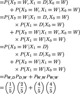
\begin{displaymath}P(X_2=W\vert X_0=W) \hspace*{230pt}
\end{displaymath}


\begin{align*}= & P(X_2=W,X_1=D \vert X_0=W)
\\
& \quad + P(X_2=W,X_1=W \vert ...
...ac{2}{5}\right)
+ \left(\frac{4}{5}\right)\left(\frac{4}{5}\right)
\end{align*}
Notice that all the entries in the last line are items in ${\bf P}$. Look at the matrix product ${\bf P}{\bf P}$:

\begin{displaymath}\left[\begin{array}{ll} \frac{3}{5} & \frac{2}{5}
\\
\\
\fr...
...ac{2}{5}
\\
\\
\frac{1}{5} & \frac{4}{5}
\end{array} \right]
\end{displaymath}

Notice that P(X2=W|X0=W) is exactly the W,W entry in ${\bf P}{\bf P}$.

General case. Define

P(n)i,j =P(Xn=j|X0=i)

Then
\begin{align*}P(X_{m+n}=j &\vert X_m=i, X_{m-1}=i_{m-1},\ldots)
\\
& = P(X_{m+n}=j\vert X_m=i)
\\
& =P(X_n=j\vert X_0=i)
\\
& = P^{(n)}_{i,j}
\end{align*}

Proof of these assertions by induction on m,n.

Example for n=2. Two bits to do:

First suppose U,V,X,Y are discrete variables. Assume
\begin{align*}P(Y=y\vert X=x,&U=u,V=v)
\\
& = P(Y=y\vert X=x)
\end{align*}
for any x,y,u,v. Then I claim
\begin{align*}P(Y=y &\vert X=x,U=u)
\\
&= P(Y=y\vert X=x)
\end{align*}
In words, if knowing both U and V doesn't change the conditional probability then knowing U alone doesn't change the conditional probability.

Proof of claim:
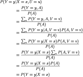
\begin{displaymath}A=\{X=x,U=u\}
\end{displaymath}

Then
\begin{align*}P(Y=y &\vert X=x,U=u)
\\
& = \frac{P(Y=y,A)}{P(A)}
\\
& = \frac{...
...}
\\
& = \frac{ P(Y=y\vert X=x)P(A)}{P(A)}
\\
&= P(Y=y\vert X=x)
\end{align*}

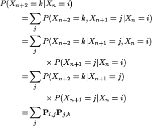
Second step: consider
\begin{align*}P(X_{n+2}& =k \vert X_n=i)
\\
= & \sum_j P(X_{n+2}=k,X_{n+1}=j\v...
...mes P(X_{n+1}=j\vert X_n=i)
\\ =& \sum_j {\bf P}_{i,j}{\bf P}_{j,k}
\end{align*}
This shows that

\begin{displaymath}P(X_{n+2}=k\vert X_n=i) = ({\bf P}^2)_{i,k}
\end{displaymath}

where ${\bf P}^2$ means the matrix product ${\bf P}{\bf P}$. Notice both that the quantity does not depend on n and that we can compute it by taking a power of ${\bf P}$.

More general version

\begin{displaymath}P(X_{n+m}=k\vert X_n=j) = ({\bf P}^m)_{j,k}
\end{displaymath}

Since ${\bf P}^n{\bf P}^m={\bf P}^{n+m}$ we get the Chapman-Kolmogorov equations:
\begin{multline*}P(X_{n+m}=k\vert X_0=i) =
\\
\sum_j P(X_{n+m}=k\vert X_n=j)P(X_n=j\vert X_0=i)
\end{multline*}

Summary: A Markov Chain has stationary n step transition probabilities which are the nth power of the 1 step transition probabilities.

Here is Maple output for the 1,2,4,8 and 16 step transition matrices for our rainfall example:

> p:= matrix(2,2,[[3/5,2/5],[1/5,4/5]]);
                      [3/5    2/5]
                 p := [          ]
                      [1/5    4/5]
> p2:=evalm(p*p):
> p4:=evalm(p2*p2):
> p8:=evalm(p4*p4):
> p16:=evalm(p8*p8):
This computes the powers (evalm understands matrix algebra).

Fact:

\begin{displaymath}\lim_{n\to\infty} {\bf P}^n = \left[
\begin{array}{cc} \frac{...
...ac{2}{3}
\\
\\
\frac{1}{3} & \frac{2}{3}
\end{array}\right]
\end{displaymath}

> evalf(evalm(p));
            [.6000000000    .4000000000]
            [                          ]
            [.2000000000    .8000000000]
> evalf(evalm(p2));
            [.4400000000    .5600000000]
            [                          ]
            [.2800000000    .7200000000]
> evalf(evalm(p4));
            [.3504000000    .6496000000]
            [                          ]
            [.3248000000    .6752000000]
> evalf(evalm(p8));
            [.3337702400    .6662297600]
            [                          ]
            [.3331148800    .6668851200]
> evalf(evalm(p16));
            [.3333336197    .6666663803]
            [                          ]
            [.3333331902    .6666668098]
Where did 1/3 and 2/3 come from?

Suppose we toss a coin $P(H)=\alpha_D$ and start the chain with Dry if we get heads and Wet if we get tails.

Then

\begin{displaymath}P(X_0=x) = \begin{cases}\alpha_D & x=\text{Dry}
\\
\alpha_W=1-\alpha_D & x=\text{Wet}
\end{cases}\end{displaymath}

and
\begin{align*}P(X_1=x) & = \sum_y P(X_1=x\vert X_0=y)P(X_0=y)
\\
& = \sum_y \alpha_y P_{y,x}
\end{align*}
Notice last line is a matrix multiplication of row vector $\alpha$ by matrix ${\bf P}$. A special $\alpha$: if we put $\alpha_D=1/3$ and $\alpha_W=2/3$ then

\begin{displaymath}\left[ \frac{1}{3} \quad \frac{2}{3} \right]
\left[\begin{ar...
...array} \right] = \left[ \frac{1}{3} \quad \frac{2}{3} \right]
\end{displaymath}

In other words if we start off P(X0=D)=1/3 then P(X1=D)=1/3and analogously for W. This means that X0 and X1 have the same distribution.

A probability vector $\alpha$ is called an initial distribution for the chain if

\begin{displaymath}P(X_0=i) = \alpha_i
\end{displaymath}

A Markov Chain is stationary if

P(X1=i) = P(X0=i)

for all i

An initial distribution is called stationary if the chain is stationary. We find that $\alpha$ is a stationary initial distribution if

\begin{displaymath}\alpha {\bf P}=\alpha
\end{displaymath}

Suppose ${\bf P}^n$ converges to some matrix ${\bf P}^\infty$. Notice that

\begin{displaymath}\lim_{n\to\infty} {\bf P}^{n-1} = {\bf P}^\infty
\end{displaymath}

and
\begin{align*}{\bf P}^\infty & = \lim {\bf P}^n
\\
& = \left[\lim {\bf P}^{n-1}\right] {\bf P}
\\
& = {\bf P}^\infty {\bf P}
\end{align*}

This proves that each row $\alpha$ of ${\bf P}^\infty$ satisfies

\begin{displaymath}\alpha = \alpha {\bf P}
\end{displaymath}

Def'n: A row vector x is a left eigenvector of A with eigenvalue $\lambda$ if

\begin{displaymath}xA=\lambda x
\end{displaymath}

So each row of ${\bf P}^\infty$ is a left eigenvector of ${\bf P}$ with eigenvalue 1.

Finding stationary initial distributions. Consider the ${\bf P}$for the weather example. The equation

\begin{displaymath}\alpha {\bf P}=\alpha
\end{displaymath}

is really
\begin{align*}\alpha_D &= 3\alpha_D/5 + \alpha_W/5
\\
\alpha_W &= 2\alpha_D/5 + 4\alpha_W/5
\end{align*}
The first can be rearranged to

\begin{displaymath}\alpha_W =2\alpha_D
\end{displaymath}

and so can the second. If $\alpha$ is to be a probability vector then

\begin{displaymath}\alpha_W+\alpha_D=1
\end{displaymath}

so we get

\begin{displaymath}1-\alpha_D=2\alpha_D
\end{displaymath}

leading to

\begin{displaymath}\alpha_D=1/3
\end{displaymath}

Some more examples:

\begin{displaymath}{\bf P}= \left[\begin{array}{cccc}
0 & 1/3 & 0 & 2/3
\\
1/3...
...\\
0 & 2/3 & 0 & 1/3
\\
2/3 & 0 & 1/3 & 0
\end{array}\right]
\end{displaymath}

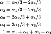
Set $\alpha{\bf P}=\alpha$ and get
\begin{align*}\alpha_1 &= \alpha_2/3+2\alpha_4/3
\\
\alpha_2 &= \alpha_1/3+2\al...
... 2\alpha_1/3+\alpha_3/3
\\
1&= \alpha_1+\alpha_2+\alpha_3+\alpha_4
\end{align*}
First plus third gives

\begin{displaymath}\alpha_1+\alpha_3=\alpha_2+\alpha_4\end{displaymath}

so both sums 1/2. Continue algebra to get

\begin{displaymath}(1/4,1/4,1/4,1/4) \, .
\end{displaymath}

p:=matrix([[0,1/3,0,2/3],[1/3,0,2/3,0],
          [0,2/3,0,1/3],[2/3,0,1/3,0]]);

               [ 0     1/3     0     2/3]
               [                        ]
               [1/3     0     2/3     0 ]
          p := [                        ]
               [ 0     2/3     0     1/3]
               [                        ]
               [2/3     0     1/3     0 ]
> p2:=evalm(p*p);
             [5/9     0     4/9     0 ]
             [                        ]
             [ 0     5/9     0     4/9]
        p2:= [                        ]
             [4/9     0     5/9     0 ]
             [                        ]
             [ 0     4/9     0     5/9]
> p4:=evalm(p2*p2):
> p8:=evalm(p4*p4):
> p16:=evalm(p8*p8):
> p17:=evalm(p8*p8*p):


> evalf(evalm(p16));
    [.5000000116 , 0 , .4999999884 , 0]
    [                                 ]
    [0 , .5000000116 , 0 , .4999999884]
    [                                 ]
    [.4999999884 , 0 , .5000000116 , 0]
    [                                 ]
    [0 , .4999999884 , 0 , .5000000116]
> evalf(evalm(p17));
    [0 , .4999999961 , 0 , .5000000039]
    [                                 ]
    [.4999999961 , 0 , .5000000039 , 0]
    [                                 ]
    [0 , .5000000039 , 0 , .4999999961]
    [                                 ]
    [.5000000039 , 0 , .4999999961 , 0]
> evalf(evalm((p16+p17)/2));
  [.2500, .2500, .2500, .2500]
  [                          ]
  [.2500, .2500, .2500, .2500]
  [                          ]
  [.2500, .2500, .2500, .2500]
  [                          ]
  [.2500, .2500, .2500, .2500]
${\bf P}^n$ doesn't converges but $({\bf P}^n+{\bf P}^{n+1})/2$ does. Next example:

\begin{displaymath}p = \left[\begin{array}{cccc}
\frac{2}{5} & \frac{3}{5}
& 0 &...
...{3}{5}
\\
0 &0 &
\frac{1}{5} & \frac{4}{5}\end{array}\right]
\end{displaymath}

Solve $\alpha{\bf P}=\alpha$:
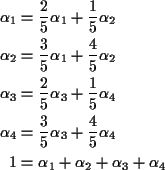
\begin{align*}\alpha_1 & = \frac{2}{5}\alpha_1+ \frac{1}{5} \alpha_2
\\
\alpha_...
...+ \frac{4}{5}\alpha_4
\\
1 & = \alpha_1+\alpha_2+\alpha_3+\alpha_4
\end{align*}
Second and fourth equations redundant. Get
\begin{align*}\alpha_2& =3\alpha_1
\\
3\alpha_3&=\alpha_4
\\
1 & = 4\alpha_1+4\alpha_3
\end{align*}

Pick $\alpha_1$ in [0,1/4]; put $\alpha_3=1/4-\alpha_1$.

\begin{displaymath}\alpha = (\alpha_1,3\alpha_1,1/4-\alpha_1,3(1/4-\alpha_1))
\end{displaymath}

solves $\alpha{\bf P}=\alpha$. So solution is not unique.

> p:=matrix([[2/5,3/5,0,0],[1/5,4/5,0,0],
            [0,0,2/5,3/5],[0,0,1/5,4/5]]);

               [2/5    3/5     0      0 ]
               [                        ]
               [1/5    4/5     0      0 ]
          p := [                        ]
               [ 0      0     2/5    3/5]
               [                        ]
               [ 0      0     1/5    4/5]
> p2:=evalm(p*p):
> p4:=evalm(p2*p2):
> p8:=evalm(p4*p4):
> evalf(evalm(p8*p8));
        [.2500000000 , .7500000000 , 0 , 0]
        [                                 ]
        [.2500000000 , .7500000000 , 0 , 0]
        [                                 ]
        [0 , 0 , .2500000000 , .7500000000]
        [                                 ]
        [0 , 0 , .2500000000 , .7500000000]
Notice that rows converge but to two different vectors:

\begin{displaymath}\alpha^{(1)} = (1/4,3/4,0,0)
\end{displaymath}

and

\begin{displaymath}\alpha^{(2)} = (0,0,1/4,3/4)
\end{displaymath}

Solutions of $\alpha{\bf P}=\alpha$ revisited? Check that

\begin{displaymath}\alpha^{(1)}{\bf P}=\alpha^{(1)}
\end{displaymath}

and

\begin{displaymath}\alpha^{(2)}{\bf P}=\alpha^{(2)}
\end{displaymath}

If $\alpha=\lambda\alpha^{(1)}+(1-\lambda)\alpha^{(2)}$( $0 \le \lambda \le 1$) then

\begin{displaymath}\alpha {\bf P}=\alpha
\end{displaymath}

so again solution is not unique. Last example:
> p:=matrix([[2/5,3/5,0],[1/5,4/5,0],
             [1/2,0,1/2]]);

                  [2/5    3/5     0 ]
                  [                 ] 
             p := [1/5    4/5     0 ]
                  [                 ]
                  [1/2     0     1/2]
> p2:=evalm(p*p):
> p4:=evalm(p2*p2):
> p8:=evalm(p4*p4):
> evalf(evalm(p8*p8));
  [.2500000000 .7500000000        0       ]
  [                                       ]
  [.2500000000 .7500000000        0       ]
  [                                       ]
  [.2500152588 .7499694824 .00001525878906]

Interpretation of examples

Basic distinguishing features: pattern of 0s in matrix ${\bf P}$.

Classification of States

State i leads to state j if ${\bf P}^n_{ij} > 0$ for some n. It is convenient to agree that ${\bf P}^0={\bf I}$ the identity matrix; thus i leads to i.

Note i leads to j and j leads to k implies i leads to k(Chapman-Kolmogorov).

States i and j communicate if i leads to j and j leads to i.

The relation of communication is an equivalence relation; it is reflexive, symmetric and transitive: if i and j communicate and j and k communicate then i and kcommunicate.

Example (+ signs indicate non-zero entries):

\begin{displaymath}{\bf P}= \left[\begin{array}{ccccc}
0& 1 & 0 & 0 &0
\\
0 & 0...
...\\
+ & 0 & 0 & + & 0
\\
0 & + & 0 & + & +
\end{array}\right]
\end{displaymath}

For this example:

$1 \leadsto 2$, $2 \leadsto 3$, $3 \leadsto 1$ so 1,2,3 are all in the same communicating class.

$4 \leadsto 1, 2, 3$ but not vice versa.

$5 \leadsto 1,2,3,4$ but not vice versa.

So the communicating classes are

\begin{displaymath}\{1,2,3\} \quad \{4\} \quad \{5\}
\end{displaymath}

A Markov Chain is irreducible if there is only one communicating class.

Notation:

\begin{displaymath}f_i=P(\exists n>0: X_n=i\vert X_0=i)
\end{displaymath}

State i is recurrent if fi=1, otherwise transient.

If fi=1 then Markov property (chain starts over when it gets back to i) means prob return infinitely many times (given started in i or given ever get to i) is 1.

Consider chain started from transient i. Let N be number of visits to state i (including visit at time 0). To return m-1 times must return once then starting over return m-1 times, then never return. So:

P(N=m) = fim-1(1-fi)

for $m=1,2,\ldots$.

N has a Geometric distribution and ${\rm E}(N) = 1/(1-f_i)$.

Another calculation:

\begin{displaymath}N=\sum_0^\infty 1(X_k=i)
\end{displaymath}

so

\begin{displaymath}{\rm E}(N) = \sum_0^\infty P(X_k=i)
\end{displaymath}

If we start the chain in state i then this is

\begin{displaymath}{\rm E}(N) = \sum_0^\infty {\bf P}^k_{ii}
\end{displaymath}

and i is transient if and only if

\begin{displaymath}\sum_0^\infty {\bf P}^k_{ii} < \infty \, .
\end{displaymath}

For last example: 4 and 5 are transient. Claim: states 1, 2 and 3 are recurrent.

Proof: argument above shows each transient state is visited only finitely many times. So: there is a recurrent state. (Note use of finite number of states.) It must be one of 1, 2 and 3. Proposition: If one state in a communicating class is recurrent then all states in the communicating class are recurrent.

Proof: Let i be the known recurrent state so

\begin{displaymath}\sum_n {\bf P}^n_{ii} = \infty
\end{displaymath}

Assume i and j communicate. Find integers m and k such that

\begin{displaymath}{\bf P}^m_{ij} > 0
\end{displaymath}

and

\begin{displaymath}{\bf P}^k_{ji} > 0
\end{displaymath}

Then

\begin{displaymath}{\bf P}^{m+n+k}_{jj} \ge {\bf P}^k_{ji} {\bf P}^n_{ii}{\bf P}^m_{ij}
\end{displaymath}

Sum RHS over n get $\infty$ so

\begin{displaymath}\sum_n {\bf P}^n_{jj} = \infty
\end{displaymath}

Proposition also means that if 1 state in a class is transient so are all.

State i has period d if d is greatest common divisor of

\begin{displaymath}\{n: {\bf P}^n_{ii} > 0\}
\end{displaymath}

If i and j are in the same class then i and j have same period. If d=1 then state i is called aperiodic; if d>1 then i is periodic.

\begin{displaymath}{\bf P}= \left[\begin{array}{ccccc}
0& 1 & 0 & 0 &0
\\
0 & 0...
...\\
0 & 0 & 0 & 0 & 1
\\
0 & 0 & 0 & 1 & 0
\end{array}\right]
\end{displaymath}

For this example $\{1,2,3\}$ is a class of period 3 states and $\{4,5\}$ a class of period 2 states.

\begin{displaymath}{\bf P}= \left[\begin{array}{ccc}
0& 1/2 & 1/2
\\
1 & 0 & 0
\\
1 & 0 & 0
\end{array}\right]
\end{displaymath}

has a single communicating class of period 2.

A chain is aperiodic if all its states are aperiodic.

Infinite State Spaces

Example: consider a sequence of independent coin tosses with probability pof Heads on a single toss. Let Xn be number of heads minus number of tails after n tosses. Put X0=0.

Xn is a Markov Chain. State space is $\Bbb Z$, the integers and

\begin{displaymath}{\bf P}_{ij} = \begin{cases}
p & j=i+1
\\
1-p & j=i-1
\\
0 & \text{otherwise}
\end{cases}\end{displaymath}

This chain has one communicating class (for $p\neq 0,1$) and all states have period 2. According to the strong law of large numbers Xn/n converges to 2p-1. If $p\neq 1/2$ this guarantees that for all large enough n $X_n \neq 0$, that is, the number of returns to 0 is not infinite. The state 0 is then transient and so all states must be transient.

For p = 1/2 the situation is different. It is a fact that

\begin{displaymath}{\bf P}^n_{00} = P(\text{\char93  H = \char93  T at time $n$})
\end{displaymath}

For n even this is the probability of exactly n/2 heads in n tosses.

Local Central Limit Theorem (normal approximation to P(-1/2 < Xn < 1/2)) (or Stirling's approximation) shows

\begin{displaymath}\sqrt{2m}P(\text{Binomial}(2m,1/2) = m) \to (2\pi)^{-1/2}
\end{displaymath}

so:

\begin{displaymath}\sum_n {\bf P}^n_{00} = \infty
\end{displaymath}

That is: 0 is a recurrent state.

Hitting Times

Start irreducible recurrent chain Xn in state i. Let Tj be first n>0 such that Xn=j. Define
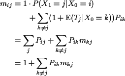
\begin{displaymath}m_{ij} = {\rm E}(T_j\vert X_0=i)
\end{displaymath}

First step analysis:
\begin{align*}m_{ij} & = 1\cdot P(X_1=j\vert X_0=i)
\\
& \qquad + \sum_{k\neq j...
...um_{k\neq j} P_{ik} m_{kj}
\\
& = 1 + \sum_{k\neq j} P_{ik} m_{kj}
\end{align*}

Example

\begin{displaymath}{\bf P}= \left[\begin{array}{cc} \frac{3}{5} & \frac{2}{5}
\\
\\
\frac{1}{5} & \frac{4}{5}
\end{array} \right]
\end{displaymath}

The equations are
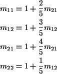
\begin{align*}m_{11} & = 1 +\frac{2}{5} m_{21}
\\
m_{12} & = 1 +\frac{3}{5} m_{...
...{21} & = 1 +\frac{4}{5} m_{21}
\\
m_{22} & = 1 +\frac{1}{5} m_{12}
\end{align*}
The second and third equations give immediately
\begin{align*}m_{12} & = \frac{5}{2}
\\
m_{21} & = 5
\end{align*}
Then plug in to the others to get
\begin{align*}m_{11} & = 3
\\
m_{22} & = \frac{3}{2}
\end{align*}

Notice stationary initial distribution is

\begin{displaymath}\left(\frac{1}{m_{11}},\frac{1}{m_{22}}\right)
\end{displaymath}

Consider fraction of time spent in state j:

\begin{displaymath}\frac{1(X_0=j)+\cdots+1(X_n=j)}{n+1}
\end{displaymath}

Imagine chain starts in chain i; take expected value.

\begin{displaymath}\frac{\sum_{r=1}^n {\bf P}^r_{ij} +1(i=j)}{n+1}
\end{displaymath}

If rows of ${\bf P}$ converge to $\pi$ then fraction converges to $\pi_j$; i.e. limiting fraction of time in state j is $\pi_j$.

Heuristic: start chain in i. Expect to return to i every mii time units. So are in state i about once every mii time units; i.e. limiting fraction of time in state iis 1/mii.

Conclusion: for an irreducible recurrent finite state space Markov chain

\begin{displaymath}\pi_i = \frac{1}{m_{ii}} \, .
\end{displaymath}

Infinite State Spaces

Previous conclusion is still right if there is a stationary initial distribution.

Example: $X_n = \text{Heads}-\text{Tails}$ after n tosses of fair coin. Equations are
\begin{align*}m_{0,0} & = 1 + \frac{1}{2}m_{1,0}+\frac{1}{2} m_{-1,0}
\\
m_{1,0} & = 1 + \frac{1}{2} m_{2,0}
\end{align*}
and many more.

Some observations:

You have to go through 1 to get to 0 from 2 so

m2,0=m2,1+m1,0

Symmetry (switching H and T):

m1,0=m-1,0

The transition probabilities are homogeneous:

m2,1=m1,0

Conclusion:


\begin{align*}m_{0,0} & = 1 + m_{1,0}
\\
& = 1+ 1 + \frac{1}{2} m_{2,0}
\\
& = 2 + m_{1,0}
\end{align*}
Notice that there are no finite solutions!

Summary of the situation:

Every state is recurrent.

All the expected hitting times mij are infinite.

All entries ${\bf P}^n_{ij}$ converge to 0.

Jargon: The states in this chain are null recurrent.

One Example

Page 229, question 21: runner goes from front or back door, prob 1/2 each. Returns front or back, prob 1/2 each. Has k pairs of shoes, wears pair if any at departure door, leaves at return door. No shoes? Barefoot. Long run fraction of time barefoot?

Solution: Let Xn be number of shoes at front door on day n. Then Xn is a Markov Chain.

Transition probabilities:

k pairs at front door on day n. Xn+1 is k if goes out back door (prob is 1/2) or out front door and back in front door (prob is 1/4). Otherwise Xn+1 is k-1.

0 < j < k pairs at front door on day n. Xn+1 is j+1if out back, in front (prob is 1/4). Xn+1 is j-1 if out front, in back. Otherwise Xn+1 is j.

0 pairs at front door on day n. Xn+1 is 0 if out front door (prob 1/2) or out back door and in back door (prob 1/4) otherwise Xn+1 is 1.

Transition matrix ${\bf P}$:


\begin{displaymath}\left[\begin{array}{cccccc}
\frac{3}{4} & \frac{1}{4} & 0 & 0...
... 0 & 0 & \cdots & \frac{1}{4} & \frac{3}{4}
\end{array}\right]
\end{displaymath}

Doubly stochastic: row sums and column sums are 1.

So $\pi_i=1/(k+1)$ for all i is stationary initial distribution.

Solution to problem: 1 day in k+1 no shoes at front door. Half of those go barefoot. Also 1 day in k+1 all shoes at front door; go barefoot half of these days. Overall go barefoot 1/(k+1) of the time.

Gambler's Ruin

Insurance company's reserves fluctuate: sometimes up, sometimes down. Ruin is event they hit 0 (company goes bankrupt). General problem. For given model of fluctuation compute probability of ruin either eventually or in next k time units.

Simplest model: gambling on Red at Casino. Bet $1 at a time. Win $1 with probability p, lose $1 with probability 1-p. Start with k dollars. Quit playing when down to $0 or up to N. Compute

\begin{displaymath}P_k = P(\text{reach $N$ before $0$})
\end{displaymath}

Xn = fortune after n plays. X0=k.

Transition matrix:

\begin{displaymath}{\bf P}=
\left[\begin{array}{cccccc}
1 & 0 & 0 & 0 &\cdots &...
...ots & \vdots
\\
0 & 0 & 0 & \cdots & 0 & 1
\end{array}\right]
\end{displaymath}

First step analysis:
\begin{align*}P_0 & =0
\\
P_i & = (1-p) P_{i-1}+pP_{i+1}
\\
P_N & = 1
\end{align*}

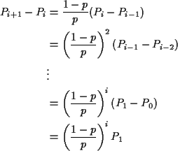
Middle equation is

pPi +(1-p)Pi = (1-p) Pi-1+pPi+1

or
\begin{align*}P_{i+1}-P_{i} &= \frac{1-p}{p} (P_{i}-P_{i-1})
\\
& = \left( \fra...
...}\right)^{i} (P_1-P_{0})
\\
& = \left( \frac{1-p}{p}\right)^{i}P_1
\end{align*}
Sum from i=0 to i=k-1 to get

\begin{displaymath}P_k = \sum_{i=0}^{k-1} \left( \frac{1-p}{p}\right)^i P_1
\end{displaymath}

or

\begin{displaymath}P_k = \frac{1-\{(1-p)/p\}^k}{1-\{(1-p)/p\}} P_1
\end{displaymath}

For k=N we get

\begin{displaymath}1=\frac{1-\{(1-p)/p\}^N}{1-\{(1-p)/p\}} P_1
\end{displaymath}

so that

\begin{displaymath}P_k = \frac{1-\{(1-p)/p\}^k}{1-\{(1-p)/p\}^N} P_1
\end{displaymath}

Notice that if p=1/2 our formulas for the sum of the geometric series are wrong. But for p=1/2 we get

Pk=kP1

so

\begin{displaymath}P_k=\frac{k}{N} \, .
\end{displaymath}

Mean time in transient states

\begin{displaymath}{\bf P}= \left[\begin{array}{cccc}
\frac{1}{2} & \frac{1}{2} ...
... & \frac{1}{4} & \frac{3}{8} & \frac{1}{8}
\end{array}\right]
\end{displaymath}

States 3 and 4 are transient. Let mi,j be the expected total number of visits to state j for chain started in i.

For i=1 or i=2 and j=3 or 4:

mij = 0

For j=1 or j=2

\begin{displaymath}m_{ij} = \infty
\end{displaymath}

For $i,j \in \{3,4\}$ first step analysis:
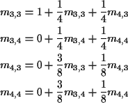
\begin{align*}m_{3,3} & = 1+ \frac{1}{4} m_{3,3} + \frac{1}{4} m_{4,3}
\\
m_{3,...
...{4,3}
\\
m_{4,4} & = 0 + \frac{3}{8} m_{3,4} + \frac{1}{8} m_{4,4}
\end{align*}

In matrix form
\begin{align*}\left[\begin{array}{cc} m_{3,3} &m_{3,4} \\ \\
m_{4,3} &m_{4,4}\e...
...ray}{cc} m_{3,3} &m_{3,4} \\ \\
m_{4,3} &m_{4,4}\end{array}\right]
\end{align*}

Translate to matrix notation:

\begin{displaymath}{\bf M} = {\bf I} + {\bf P}_T {\bf M}
\end{displaymath}

where $\bf I$ is the identity, $\bf M$ is the matrix of means and ${\bf P}_T$ the part of the transition matrix corresponding to transient states.

Solution is

\begin{displaymath}{\bf M} = ({\bf I} - {\bf P}_T)^{-1}
\end{displaymath}

In our case

\begin{displaymath}{\bf I} - {\bf P}_T =
\left[\begin{array}{rr} \frac{3}{4} &...
...rac{1}{4} \\ \\
-\frac{3}{8} & \frac{7}{8}
\end{array}\right]
\end{displaymath}

so that

\begin{displaymath}{\bf M} = \left[\begin{array}{rr} \frac{14}{9} & -\frac{4}{9} \\ \\
-\frac{2}{3} & \frac{4}{3}
\end{array}\right]
\end{displaymath}

Poisson Processes

Particles arriving over time at a particle detector. Several ways to describe most common model.

Approach 1: numbers of particles arriving in an interval has Poisson distribution, mean proportional to length of interval, numbers in several non-overlapping intervals independent.

For s<t, denote number of arrivals in (s,t] by N(s,t). Model is

1.
N(s,t) has a Poisson $(\lambda(t-s))$ distribution.

2.
For $ 0 \le s_1 < t_1 \le s_2 < t_2 \cdots \le s_k < t_k$ the variables $N(s_i,t_i);i=1,\ldots,k$ are independent.

Approach 2:

Let $0 < S_1 <S_2 < \cdots $ be the times at which the particles arrive.

Let Ti = Si-Si-1 with S0=0 by convention.

Then $T_1,T_2,\ldots$are independent Exponential random variables with mean $1/\lambda$.

Note $P(T_i > x) =e^{-\lambda x}$ is called survival function of Ti.

Approaches are equivalent. Both are deductions of a model based on local behaviour of process.

Approach 3: Assume:

1.
given all the points in [0,t] the probability of 1 point in the interval (t,t+h] is of the form

\begin{displaymath}\lambda h +o(h)
\end{displaymath}

2.
given all the points in [0,t] the probability of 2 or more points in interval (t,t+h] is of the form

o(h)

All 3 approaches are equivalent. I show: 3 implies 1, 1 implies 2 and 2 implies 3. First explain o, O.

Notation: given functions f and g we write

f(h) = g(h) +o(h)

provided

\begin{displaymath}\lim_{h \to 0} \frac{f(h)-g(h)}{h} = 0
\end{displaymath}

[Aside: if there is a constant M such that

\begin{displaymath}\limsup_{h \to 0} \left\vert\frac{f(h)-g(h)}{h}\right\vert \le M
\end{displaymath}

we say

f(h) = g(h)+O(h)

Notation due to Landau. Another form is

f(h) = g(h)+O(h)

means there is $\delta>0$ and M s.t. for all $\vert h\vert<\delta$

\begin{displaymath}\vert f(h)-g(h) \vert\le M h
\end{displaymath}

Idea: o(h) is tiny compared to h while O(h) is (very) roughly the same size as h.]

Model 3 implies 1: Fix t, define ft(s) to be conditional probability of 0 points in (t,t+s] given value of process on [0,t].

Derive differential equation for f. Given process on [0,t] and 0 points in (t,t+s] probability of no points in (t,t+s+h] is

\begin{displaymath}f_{t+s}(h) = 1-\lambda h+o(h)
\end{displaymath}

Given the process on [0,t] the probability of no points in (t,t+s] is ft(s). Using P(AB|C)=P(A|BC)P(B|C) gives
\begin{align*}f_t(s+h) & = f_t(s)f_{t+s}(h)
\\
& = f_t(s)(1-\lambda h +o(h))
\end{align*}
Now rearrange, divide by h to get

\begin{displaymath}\frac{f_t(s+h) - f_t(s)}{h} = \lambda f_t(s) +\frac{o(h)}{h}
\end{displaymath}

Let $h \to 0$ and find

\begin{displaymath}\frac{\partial f_t(s)}{\partial s} = -\lambda f_t(s)
\end{displaymath}

Differential equation has solution

\begin{displaymath}f_t(s) = f_t(0) \exp(-\lambda s) = \exp(-\lambda s)\, .
\end{displaymath}

Notice: survival function of exponential rv..

General case:

Notation: N(t) =N(0,t).

N(t) is a non-decreasing function of t. Let

Pk(t) = P(N(t)=k)

Evaluate Pk(t+h) by conditioning on $N(s);0 \le s < t$ and N(t)=j.

Given N(t)=j probability that N(t+h) = k is conditional probability of k-j points in (t,t+h].

So, for $j\le k-2$:
\begin{multline*}P(N(t+h)=k\vert N(t) = j, N(s), 0 \le s < t)
\\ =o(h)
\end{multline*}
For j=k-1 we have
\begin{multline*}P(N(t+h)= k\vert N(t) = k-1, N(s), 0 \le s < t)
\\
= \lambda h + o(h)
\end{multline*}
For j=k we have
\begin{multline*}P(N(t+h)= k\vert N(t) = k, N(s), 0 \le s < t)
\\
= 1-\lambda h + o(h)
\end{multline*}

N is increasing so only consider $j\le k$.
\begin{align*}P_k(t+h) & = \sum_{j=0}^k P(N(t+h)=k\vert N(t) = j) P_j(t)
\\
& = P_k(t) (1-\lambda h) +\lambda h P_{k-1}(t) + o(h)
\end{align*}
Rearrange, divide by h and let $h \to 0$ t get

\begin{displaymath}P_k^\prime(t) = -\lambda P_k(t) + \lambda P_{k-1}(t)
\end{displaymath}

For k=0 the term Pk-1 is dropped and

\begin{displaymath}P^\prime_0(t) = \lambda P_0(t)
\end{displaymath}

Using P0(0)=1 we get

\begin{displaymath}P_0(t) = e^{-\lambda t}
\end{displaymath}

Put this into the equation for k=1 to get

\begin{displaymath}P_1^\prime(t) = -\lambda P_1(t) +\lambda e^{-\lambda t}
\end{displaymath}

Multiply by $ e^{\lambda t}$ to see

\begin{displaymath}\left(e^{\lambda t}P_1(t)\right)^\prime = \lambda
\end{displaymath}

With P1(0)=0 we get

\begin{displaymath}P_1(t) = \lambda t e^{-\lambda t}
\end{displaymath}

For general k we have Pk(0)=0 and

\begin{displaymath}\left(e^{\lambda t}P_k(t)\right)^\prime = \lambda e^{\lambda t}P_{k-1}(t)
\end{displaymath}

Check by induction that

\begin{displaymath}e^{\lambda t}P_k(t) = (\lambda t)^k/k!
\end{displaymath}

Hence: N(t) has Poisson $(\lambda t)$ distribution.

Similar ideas permit proof of
\begin{multline*}P(N(s,t)=k\vert N(u); 0 \le u \le s)
\\
= \frac{\left\{\lambda(t-s)\right\}^k e^{-\lambda}}{k!}
\end{multline*}
From which (by induction) we can prove that Nhas independent Poisson increments.

Exponential Interarrival Times

If N is a Poisson Process we define $T_1,T_2,\ldots$to be the times between 0 and the first point, the first point and the second and so on.

Fact: $T_1,T_2,\ldots$ are iid exponential rvs with mean $1/\lambda$.

We already did T1 rigorously. The event T>t is exactly the event N(t)=0. So

\begin{displaymath}P(T>t) = \exp(-\lambda t)
\end{displaymath}

which is the survival function of an exponential rv.

I do case of T1,T2. Let t1,t2 be two positive numbers and s1=t1, s2=t1+t2. The event

\begin{displaymath}\{t_1 < T_1 \le t_1+\delta_1\} \cap \{t_2 < T_2 \le t_2+\delta_2\} \, .
\end{displaymath}

This is almost the same as the intersection of the four events:
\begin{align*}N(0,t_1]&=0
\\
N(t_1,t_1+\delta_1] & = 1
\\
N(t_1+\delta_1,t_1+\delta_1+t_2] & =0
\\
N(s_2+\delta_1,s_2+\delta_1+\delta_2] & = 1
\end{align*}
which has probability

\begin{displaymath}e^{-\lambda t_1} \times \lambda\delta_1 e^{-\lambda \delta_1}...
... e^{-\lambda t_2} \times \lambda\delta_2 e^{-\lambda \delta_2}
\end{displaymath}

Divide by $\delta_1\delta_2$ and let $\delta_1$ and $\delta_2$ go to 0 to get joint density of T1,T2 is

\begin{displaymath}e^{-\lambda t_1}e^{-\lambda t_2}
\end{displaymath}

which is the joint density of two independent exponential variates.

More rigor:

First step: Compute

\begin{displaymath}P( 0 < S_1 \le s_1 < S_2 \le s_2 \cdots < S_k \le s_k)
\end{displaymath}

This is just the event of exactly 1 point in each interval (si-1,si] for $i=1,\ldots,k-1$ (s0=0) and at least one point in (sk-1,sk] which has probability

\begin{displaymath}\prod_1^{k-1} \left\{\lambda(s_i-s_{i-1})e^{-\lambda(s_i-s_{i-1})}\right\}
\left(1-e^{-\lambda(s_k-s_{k-1})}\right)
\end{displaymath}

Second step: write this in terms of joint cdf of $S_1,\ldots,S_k$. I do k=2:
\begin{multline*}P( 0 < S_1 \le s_1 < S_2 \le s_2) \\ =
F_{S_1,S_2}(s_1,s_2)-F_{S_1,S_2}(s_1,s_1)
\end{multline*}
Notice tacit assumption s1 < s2.

Differentiate twice, that is, take

\begin{displaymath}\frac{\partial^2}{\partial s_1\partial s_2}
\end{displaymath}

to get
\begin{multline*}f_{S_1,S_2}(s_1,s_2)\\ = \frac{\partial^2}{\partial s_1\partial...
...ambda s_1 e^{-\lambda s_1} \left(1-e^{-\lambda (s_2-s_1)}\right)
\end{multline*}
Simplify to

\begin{displaymath}\lambda^2 e^{-\lambda s_2}
\end{displaymath}

Recall tacit assumption to get

\begin{displaymath}f_{S_1,S_2}(s_1,s_2) =\lambda^2 e^{-\lambda s_2} 1(0 < s_1 < s_2)
\end{displaymath}

That completes the first part.

Now compute the joint cdf of T1,T2 by
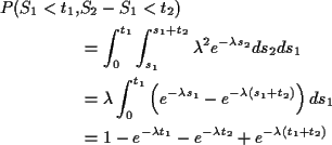
FT1,T2(t1,t2) = P(S1 < t1, S2-S1 <t2)

This is
\begin{align*}P(S_1 < t_1,& S_2-S_1 <t_2)
\\
& = \int_0^{t_1} \int_{s_1}^{s_1+...
...
& = 1-e^{-\lambda t_1} - e^{-\lambda t_2} + e^{-\lambda(t_1+t_2)}
\end{align*}
Differentiate twice to get

\begin{displaymath}f_{T_1,T_2}(t_1,t_2) = \lambda e^{-\lambda t_1} \lambda e^{-\lambda t_2}
\end{displaymath}

which is the joint density of two independent exponential random variables.

Summary so far:

Have shown:

Instantaneous rates model implies independent Poisson increments model implies independent exponential interarrivals.

Next: show independent exponential interarrivals implies the instantaneous rates model.

Suppose $T_1,\ldots$ iid exponential rvs with means $1/\lambda$. Define Nt by Nt=k if and only if

\begin{displaymath}T_1+\cdots+T_k \le t \le T_1+\cdots +T_{k+1}
\end{displaymath}

Let A be the event $N(s)=n(s) ;0 < s \le t$. We are to show

\begin{displaymath}P(N(t,t+h] = 1\vert N(t)=k,A) = \lambda h + o(h)
\end{displaymath}

and

\begin{displaymath}P(N(t,t+h] \ge 2\vert N(t)=k,A) = o(h)
\end{displaymath}

If n(s) is a possible trajectory consistent with N(t) = kthen n has jumps at points

\begin{displaymath}t_1,t_1+t_2, \ldots,t_1+\cdots+t_k < t
\end{displaymath}

and at no other points in (0,t].

So given $N(s)=n(s) ;0 < s \le t$with n(t)=k we are essentially being given

\begin{displaymath}T_1=t_1,\ldots,T_k=t_k, T_{k+1}> t-s_k
\end{displaymath}

(using $s_k = t_1+\cdots+t_k$) and asked the conditional probabilty in the first case of the event B given by

\begin{displaymath}t-s_k <T_{k+1}\le t-s_k+h < T_{k+2}+T_{k+1}\, .
\end{displaymath}

Conditioning on $T_1,\ldots,T_k$ irrelevant (independence).


\begin{align*}P(N(t,t+h] = 1\vert& N(t)=k,A) /h
\\
& = P(B\vert T_{k+1}> t-s_k)/h
\\
& = \frac{P(B) }{he^{-\lambda(t-s_k)}}
\end{align*}
The numerator may be evaluated by integration:

\begin{displaymath}P(B) = \int_{t-s_k}^{t-s_k+h} \int_{t-s_k+h - s_1}^\infty \lambda^2 e^{-\lambda(s_1+s_2)} ds_2ds_1
\end{displaymath}

Let $h \to 0$ to get the limit

\begin{displaymath}P
(N(t,t+h] = 1\vert N(t)=k,A) /h \to \lambda
\end{displaymath}

as required.

The computation of

\begin{displaymath}\lim_{h\to 0} P(N(t,t+h] \ge 2\vert N(t)=k,A) /h
\end{displaymath}

is similar.

Properties of exponential rvs

Convolution: If $T_1,\ldots,T_n$ iid Exponential$(\lambda)$then $S_n=T_1+\cdots+T_n$ has a Gamma $(n,\lambda)$ distribution. Density of Sn is

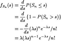
\begin{displaymath}f_{S_n}(s) = \lambda (\lambda s)^{n-1} e^{-\lambda s} / n!
\end{displaymath}

for s>0.

Proof:
\begin{align*}P(S_n>s)& = P(N(0,s] \le n)
\\
& = (\lambda s)^n e^{-\lambda s}/n!
\end{align*}
Then
\begin{align*}f_{S_n}(s) & = \frac{d}{ds} P(S_n \le s)
\\
& = \frac{d}{ds}\left...
...^{-\lambda s}/n!
\\
& = \lambda (\lambda s)^{n-1}e^{-\lambda s}/n!
\end{align*}

Extreme Values: If $X_1,\ldots,X_n$ are independent exponential rvs with means $1/\lambda_1,\ldots,1/\lambda_n$then $Y = \min\{X_1,\ldots,X_n\}$ has an exponential distribution with mean

\begin{displaymath}\frac{1}{\lambda_1+\cdots+\lambda_n}
\end{displaymath}

Proof:
\begin{align*}P(Y > y) & = P(\forall k X_k>y)
\\
& = \prod e^{-\lambda_k y}
\\
& = e^{-\sum\lambda_k y}
\end{align*}

Memoryless Property: conditional distribution of X-x given $X \ge x$ is exponential if X has an exponential distribution.

Proof:
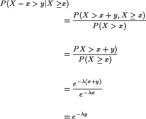
\begin{align*}P(X-x>y\vert X\ge& x)
\\
& = \frac{P(X>x+y,X\ge x)}{P(X>x)}
\\
\...
...\frac{e^{-\lambda(x+y)}}{e^{-\lambda x}}
\\
\\
& = e^{-\lambda y}
\end{align*}

Hazard Rates

The hazard rate, or instantaneous failure rate for a positive random variable T with density f and cdf F is

\begin{displaymath}r(t) = \lim_{\delta\to 0} \frac{P(t < T\le t+\delta \vert T \ge t)}{\delta}
\end{displaymath}

This is just

\begin{displaymath}r(t) = \frac{f(t)}{1-F(t)}
\end{displaymath}

For an exponential random variable with mean $1/\lambda$ this is

\begin{displaymath}h(t) = \frac{ \lambda e^{-\lambda t}}{e^{-\lambda t}} = \lambda
\end{displaymath}

The exponential distribution has constant failure rate.

Weibull random variables have density

\begin{displaymath}f(t\vert\lambda,\alpha) = \lambda(\lambda t)^{\alpha-1}e^{- (\lambda t)^\alpha}
\end{displaymath}

for t>0. The corresponding survival function is

\begin{displaymath}1-F(t) = e^{- (\lambda t)^\alpha}
\end{displaymath}

and the hazard rate is

\begin{displaymath}r(t) = \lambda(\lambda t)^{\alpha-1}
\end{displaymath}

which is increasing for $\alpha>1$, decreasing for $\alpha<1$. For $\alpha=1$this is the exponential distribution.

Since

\begin{displaymath}r(t) = \frac{dF(t)/dt}{1-F(t)} =-\frac{d\log(1-F(t))}{dt}
\end{displaymath}

we can integrate to find

\begin{displaymath}1-F(t) = \exp\{ -\int_0^t r(s) ds\}
\end{displaymath}

so that r determines F and f.

Richard Lockhart
2000-10-16