Course outline:
Example 1: Three cards: one red on both sides, one black on both sides, one black on one side, red on the other. Shuffle, pick card at random. Side up is Black. What is the probability the side down is Black?
Solution: To do this carefully, enumerate sample space,
![]() , of all possible outcomes. Six sides to the three cards.
Label three red sides 1, 2, 3 with sides 1, 2 on the all red card (card
# 1).
Label three black sides 4, 5, 6 with 3, 4 on opposite sides of mixed
card (card #2). Define some events:
, of all possible outcomes. Six sides to the three cards.
Label three red sides 1, 2, 3 with sides 1, 2 on the all red card (card
# 1).
Label three black sides 4, 5, 6 with 3, 4 on opposite sides of mixed
card (card #2). Define some events:
 side side |
||
 side showing is black side showing is black |
||
 card card |
One representation
 . Then
 ,
,
 ,
,
 and so on.
Modelling: assumptions about some probabilities; deduce probabilities of other events. In example simplest model is
Apply two rules:
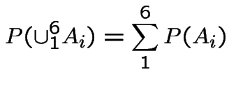 and
and
 ,
,

 . (Of course
Definition of conditional probability:

Example 2: Monte Hall, Let's Make a Deal. Monte shows you 3 doors. Prize hidden behind one. You pick a door. Monte opens a door you didn't pick; shows you no prize; offers to let you switch to the third door. Do you switch?
Sample space: typical element is  where
where ![]() is number
of door with prize,
is number
of door with prize, ![]() is number of your first pick and
is number of your first pick and ![]() is
door Monte opens with no prize.
is
door Monte opens with no prize.
| (1,1,2) | (1,1,3) | (1,2,3) | (1,3,2) |
| (2,1,3) | (2,2,1) | (2,2,3) | (2,3,1) |
| (3,1,2) | (3,2,1) | (3,3,1) | (3,3,2) |
Model? Traditionally we define events like
 Prize behind door Prize behind door |
||
 You choose door You choose door |
 . We
are assuming we have no prior reason to suppose
Monte favours one door. But these and all other
probabilities depend on the behaviour of people
so are open to discussion.
The event ![]() , that you lose if you switch is
, that you lose if you switch is


 |
 |
|
 |
||
 |
||
 |
||
 |
||
So the event you win by switching has probability 2/3 and you should switch.
Usual phrasing of problem. You pick 1, Monte shows 3. Should
you take 2? Let ![]() be rv
be rv ![]() door Monte
shows you. Question:
door Monte
shows you. Question:

Modelling assumptions do not determine this; it depends on Monte's method for choosing door to show when he has a choice. Two simple cases:


Use Bayes' rule:


For case 1 we get


Notice that in case 2 if we pick door 1 and Monte shows us door 2 we should definitely switch. Notice also that it would be normal to assume that Monte used the case 1 algorithm to pick the door to show when he has a choice; otherwise he is giving the contestant information. If the contestant knows Monte is using algorithm 2 then by switching if door 2 is shown and not if door 3 is shown he wins 2/3 of the time which is as good as the always switch strategy.
Example 3: Survival of family names. Traditionally: family name follows sons. Given man at end of 20th century. Probability descendant (male) with same last name alive at end of 21st century? or end of 30th century?
Simplified model: count generations not years. Compute probability,
of survival of name for ![]() generations.
generations.
Technically easier to compute ![]() , probability of extinction by
generation
, probability of extinction by
generation ![]() .
.
Useful rvs:
 # of male children of first man
 # of male children in generation $k$
 :
:

 . Let
. Let
 |
 child child |
|
in  generations generations |

 are independent. In other words: one son's
descendants don't affect other sons' descendants.
 is
is  .
In other words: sons are just like the parent.
 .
.
 |
||
 |
||
 |
||
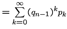 |


 so that the limit of
the
  , must exist and (because
Geometric Distribution: Assume

Then
 |
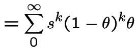 |
|
![$\displaystyle = \theta \sum_0^\infty \left[s(1-\theta)\right]^k$](img87.gif) |
||
 |
 to get
![$\displaystyle s[1-s(1-\theta)]=\theta
$](img90.gif)


 the only root which is a probability is 1 and
 . If
. If
 then in fact
 .
.
Binomial( ): If
): If

 |
 |
|
 |
 has two roots. One is 1. The other is
less than 1 if and only if
 .
.
Poisson(![]() ): Now
): Now


 has two roots. One is 1. The other
is less than 1 if and only if
 .
.
Important Points:
Example 3: Mean values
![]() = total number of sons in generation
= total number of sons in generation ![]() .
.
 for convenience.
Compute
 .
.
Recall definition of expected value:
If ![]() is discrete then
is discrete then

If ![]() is absolutely continuous then
is absolutely continuous then

Theorem: If  ,
, ![]() has density
has density ![]() then
then

Key properties of ![]() :
:
1: If  then
then
 . Equals iff
 .
.
2:
 .
.
3: If
 then
then

4:
 .
.
Conditional Expectations
If ![]() ,
, ![]() , two discrete random variables then
, two discrete random variables then

Extension to absolutely continuous case:
Joint pmf of ![]() and
and ![]() is defined as
is defined as


 is
is


 have joint density
  then
then 
Example:

 |
 |
|
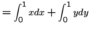 |
||
 |
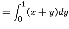
The marginal density of ![]() is, for
is, for
 .
.
 |
 |
|
 |
||
 |
For ![]() not in
not in ![$ [0,1]$](img142.gif) the integral is 0 so
the integral is 0 so

Conditional Densities
If ![]() and
and ![]() have joint density
have joint density
 then
we define the conditional density of
 ![]() given
given ![]() by
analogy with our interpretation of densities. We take limits:
by
analogy with our interpretation of densities. We take limits:


Going back to our interpretation of joint densities and ordinary densities we see that our definition is just

 as the joint density and to
  as
the marginal density of
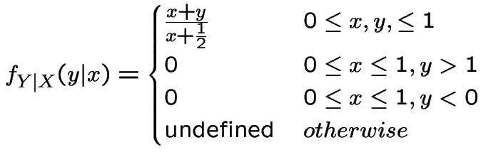
Example: For ![]() of previous example conditional density
of
of previous example conditional density
of ![]() given
given ![]() defined only for
defined only for
 :
:
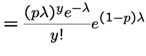
 random variable. Observe
 |
 |
|
 |
||
 |
WARNING: in sum
 is required and
 ![]() ,
, ![]() integers
so sum really runs from
integers
so sum really runs from ![]() to
to ![]()
 |
![$\displaystyle = \frac{(p\lambda)^ye^{-\lambda}}{y!} \sum_{x=y}^\infty \frac{\left[(1-p)\lambda\right]^{x-y}}{(x-y)!}$](img163.gif) |
|
![$\displaystyle = \frac{(p\lambda)^ye^{-\lambda}}{y!}\sum_0^\infty \frac{\left[(1-p)\lambda\right]^{k}}{k!}$](img164.gif) |
||
 |
||
 |
Conditional Expectations
If ![]() and
and ![]() are continuous random variables with joint density
are continuous random variables with joint density
 we define:

Key properties of conditional expectation
1: If  then
then
 . Equals iff
 .
.
2:
 .
.
3: If ![]() and
and ![]() are independent then
are independent then

4:
 .
.
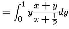
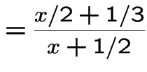
Example:

 :
:

 ,
,
 |
 |
|
 |
Computing expectations by conditioning:
Notation:
 is the function of
 ![]() you get by
working out
you get by
working out
 , getting a formula in
 ![]() and replacing
and replacing
![]() by
by ![]() . This makes
. This makes
 a random variable.
Properties:
1:
 .
.
2: If ![]() and
and ![]() are independent then
are independent then

3:
 .
.
4:
![$ {\rm E}\left[{\rm E}(Y\vert X)\right] = {\rm E}(Y) $](img184.gif) (compute average
holding
(compute average
holding ![]() fixed first, then average over
fixed first, then average over ![]() ).
).
In example:


 |
![$\displaystyle = {\rm E}\left[{\rm E}(Z_n\vert X)\right]$](img188.gif) |
|
![$\displaystyle = {\rm E}\left[ X{\rm E}(Z_{n-1})\right]$](img189.gif) |
||
 |
||
 |
||
 |
||
 |
||
 |
||
 |
For  expect exponential decay. For
  exponential
growth (if not extinction).
We have reviewed the following definitions:
![$ [0,1]$](img142.gif) satisfying:
satisfying:
 and
and
 .
.
 pairwise disjoint
(
 )
)

 discrete:


 continuous:
 ; probabilities are double integrals


 is previous with
Tactics:
 is known.
 is a partition
then

Tactics for expected values:

![$\displaystyle {\rm E}\left[{\rm E}(Y\vert X)\right] = {\rm E}(Y)
$](img222.gif)
Last names example has following structure: if, at generation
![]() there are
there are ![]() individuals then number of sons in
next generation has distribution of sum of
individuals then number of sons in
next generation has distribution of sum of ![]() independent
copies of the random variable
independent
copies of the random variable ![]() which is number of sons I have.
This distribution does not depend on
which is number of sons I have.
This distribution does not depend on ![]() , only on value
, only on value ![]() of
of ![]() .
Call
.
Call ![]() a Markov Chain.
a Markov Chain.
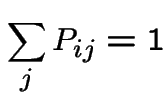
Ingredients of a Markov Chain:
 of random variables whose values
are all in
 for
for  .
.
 and
and
The stochastic process
 is called a
Markov chain if

 and for all
  . Usually used with

 .
.
The matrix ![]() is called a transition matrix.
is called a transition matrix.
Example: If ![]() in the last names example has
a Poisson
in the last names example has
a Poisson distribution then given
  ,
,
 is like sum of
 ![]() independent Poisson
independent Poisson rvs which has a Poisson(
![]() ) distribution.
So
) distribution.
So
![$\displaystyle {\bf P}= \left[\begin{array}{llll}
1 & 0 & 0 & \cdots
\\
e^{-\l...
...\lambda} &
\cdots
\\
\vdots &
\vdots &
\vdots &
\ddots
\end{array}\right]
$](img239.gif)
Example: Weather: each day is dry (D) or wet (W).
 is weather on day n.
Suppose dry days tend to be followed by dry days, say 3 times in 5 and wet days by wet 4 times in 5.
Markov assumption: yesterday's weather irrelevant to prediction of tomorrow's given today's.
Transition Matrix:
![$\displaystyle {\bf P}= \left[\begin{array}{cc} \frac{3}{5} & \frac{2}{5}
\\
\\
\frac{1}{5} & \frac{4}{5}
\end{array} \right]
$](img241.gif)
Now suppose it's wet today. P(wet in 2 days)?

 |
||
 |
||
 |
||
 |
||
 |
||
 |
||
 |
||
 |
||
 |
||
 |
||
 |
||
 |
![$\displaystyle \left[\begin{array}{ll} \frac{3}{5} & \frac{2}{5}
\\
\\
\frac...
...} & \frac{14}{25}
\\
\\
\frac{7}{25} & \frac{18}{25}
\end{array} \right]
=
$](img254.gif)
 is exactly the
  entry
in
General case. Define

 |
 |
|
 |
||
 |
||
 |
||
 |
Proof of these assertions by induction on  .
.
Example for ![]() . Two bits to do:
. Two bits to do:
First suppose  are discrete variables.
Assume
 |
 |
|
 |
 . Then I claim
 |
 |
|
 |
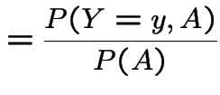
Proof of claim:

 |
 |
|
 |
||
 |
||
 |
||
 |
||
 |
||
 |
||
 |
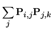
Second step: consider
 |
 |
|
 |
||
 |
||
 |
||
 |
||
 |
||
 |

More general version


Summary: A Markov Chain has stationary ![]() step transition
probabilities which are the
step transition
probabilities which are the ![]() th power of the 1 step transition
probabilities.
th power of the 1 step transition
probabilities.
Here is Maple output for the 1,2,4,8 and 16 step transition matrices for our rainfall example:
> p:= matrix(2,2,[[3/5,2/5],[1/5,4/5]]);
                      [3/5    2/5]
                 p := [          ]
                      [1/5    4/5]
> p2:=evalm(p*p):
> p4:=evalm(p2*p2):
> p8:=evalm(p4*p4):
> p16:=evalm(p8*p8):
This computes the powers ( evalm understands
matrix algebra).
Fact:
![\begin{displaymath}
\lim_{n\to\infty} {\bf P}^n = \left[
\begin{array}{cc} \frac...
...{2}{3}
\\
\\
\frac{1}{3} & \frac{2}{3}
\end{array}\right]
\end{displaymath}](img294.gif)
> evalf(evalm(p));
            [.6000000000    .4000000000]
            [                          ]
            [.2000000000    .8000000000]
> evalf(evalm(p2));
            [.4400000000    .5600000000]
            [                          ]
            [.2800000000    .7200000000]
> evalf(evalm(p4));
            [.3504000000    .6496000000]
            [                          ]
            [.3248000000    .6752000000]
> evalf(evalm(p8));
            [.3337702400    .6662297600]
            [                          ]
            [.3331148800    .6668851200]
> evalf(evalm(p16));
            [.3333336197    .6666663803]
            [                          ]
            [.3333331902    .6666668098]
Where did  and
and  come from?
Suppose we toss a coin
 and start the
chain with Dry if we get heads and Wet if we get
tails.
Then

 |
 |
|
 |
 and
and
 then
then
![$\displaystyle \left[ \frac{1}{3} \quad \frac{2}{3} \right]
\left[\begin{array}{...
...frac{4}{5}
\end{array} \right] = \left[ \frac{1}{3} \quad \frac{2}{3} \right]
$](img304.gif)
 then
then
 and analogously for
  and
and  have the
same distribution.
A probability vector ![]() is called an initial distribution for
the chain if
is called an initial distribution for
the chain if

A Markov Chain is stationary if

An initial distribution is called stationary if the chain is
stationary. We find that ![]() is a stationary initial distribution
if
is a stationary initial distribution
if

Suppose ![]() converges to some matrix
converges to some matrix
![]() . Notice that
. Notice that

 |
 |
|
![$\displaystyle = \left[\lim {\bf P}^{n-1}\right] {\bf P}$](img318.gif) |
||
 |
This proves that each row ![]() of
of
![]() satisfies
satisfies

Def'n: A row vector ![]() is a left eigenvector of
is a left eigenvector of ![]() with
eigenvalue
with
eigenvalue ![]() if
if

So each row of
![]() is a left eigenvector of
is a left eigenvector of ![]() with eigenvalue
with eigenvalue ![]() .
.
Finding stationary initial distributions. Consider the ![]() for the weather example. The equation
for the weather example. The equation

 |
 |
|
 |
 |


![$\displaystyle {\bf P}= \left[\begin{array}{cccc}
0 & 1/3 & 0 & 2/3
\\
1/3&0 & 2/3 & 0
\\
0 & 2/3 & 0 & 1/3
\\
2/3 & 0 & 1/3 & 0
\end{array}\right]
$](img331.gif)
 |
||
 |
||
 |
||
 |
||
 |


p:=matrix([[0,1/3,0,2/3],[1/3,0,2/3,0],
          [0,2/3,0,1/3],[2/3,0,1/3,0]]);

               [ 0     1/3     0     2/3]
               [                        ]
               [1/3     0     2/3     0 ]
          p := [                        ]
               [ 0     2/3     0     1/3]
               [                        ]
               [2/3     0     1/3     0 ]
> p2:=evalm(p*p);
             [5/9     0     4/9     0 ]
             [                        ]
             [ 0     5/9     0     4/9]
        p2:= [                        ]
             [4/9     0     5/9     0 ]
             [                        ]
             [ 0     4/9     0     5/9]
> p4:=evalm(p2*p2):
> p8:=evalm(p4*p4):
> p16:=evalm(p8*p8):
> p17:=evalm(p8*p8*p):
> evalf(evalm(p16));
    [.5000000116 , 0 , .4999999884 , 0]
    [                                 ]
    [0 , .5000000116 , 0 , .4999999884]
    [                                 ]
    [.4999999884 , 0 , .5000000116 , 0]
    [                                 ]
    [0 , .4999999884 , 0 , .5000000116]
> evalf(evalm(p17));
    [0 , .4999999961 , 0 , .5000000039]
    [                                 ]
    [.4999999961 , 0 , .5000000039 , 0]
    [                                 ]
    [0 , .5000000039 , 0 , .4999999961]
    [                                 ]
    [.5000000039 , 0 , .4999999961 , 0]
> evalf(evalm((p16+p17)/2));
  [.2500, .2500, .2500, .2500]
  [                          ]
  [.2500, .2500, .2500, .2500]
  [                          ]
  [.2500, .2500, .2500, .2500]
  [                          ]
  [.2500, .2500, .2500, .2500]
 does.
Next example:
![$\displaystyle p = \left[\begin{array}{cccc}
\frac{2}{5} & \frac{3}{5}
& 0 &0
\\...
...ac{2}{5} & \frac{3}{5}
\\
0 &0 &
\frac{1}{5} & \frac{4}{5}\end{array}\right]
$](img346.gif)
 |
||
 |
||
 |
||
 |
||
 |
 |
||
 |
 |
|
 |
Pick ![]() in
in ![$ [0,1/4]$](img356.gif) ;
put
;
put
 .
.

> p:=matrix([[2/5,3/5,0,0],[1/5,4/5,0,0],
            [0,0,2/5,3/5],[0,0,1/5,4/5]]);

               [2/5    3/5     0      0 ]
               [                        ]
               [1/5    4/5     0      0 ]
          p := [                        ]
               [ 0      0     2/5    3/5]
               [                        ]
               [ 0      0     1/5    4/5]
> p2:=evalm(p*p):
> p4:=evalm(p2*p2):
> p8:=evalm(p4*p4):
> evalf(evalm(p8*p8));
        [.2500000000 , .7500000000 , 0 , 0]
        [                                 ]
        [.2500000000 , .7500000000 , 0 , 0]
        [                                 ]
        [0 , 0 , .2500000000 , .7500000000]
        [                                 ]
        [0 , 0 , .2500000000 , .7500000000]
Notice that rows converge but to two different vectors:


 (
(
 ) then

> p:=matrix([[2/5,3/5,0],[1/5,4/5,0],
             [1/2,0,1/2]]);

                  [2/5    3/5     0 ]
                  [                 ]
             p := [1/5    4/5     0 ]
                  [                 ]
                  [1/2     0     1/2]
> p2:=evalm(p*p):
> p4:=evalm(p2*p2):
> p8:=evalm(p4*p4):
> evalf(evalm(p8*p8));
  [.2500000000 .7500000000        0       ]
  [                                       ]
  [.2500000000 .7500000000        0       ]
  [                                       ]
  [.2500152588 .7499694824 .00001525878906]
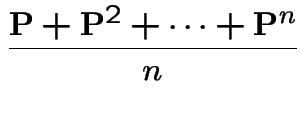
Basic distinguishing features: pattern of 0s in matrix ![]() .
.
State ![]() leads to state
leads to state ![]() if
if
 for some
 ![]() .
It is convenient to agree that
.
It is convenient to agree that
![]() the identity matrix;
thus
the identity matrix;
thus ![]() leads to
leads to ![]() .
.
Note ![]() leads to
leads to ![]() and
and ![]() leads to
leads to ![]() implies
implies ![]() leads to
leads to ![]() (Chapman-Kolmogorov).
(Chapman-Kolmogorov).
States ![]() and
and ![]() communicate if
communicate if ![]() leads to
leads to ![]() and
and ![]() leads
to
leads
to ![]() .
.
The relation of communication is an equivalence relation; it
is reflexive, symmetric and transitive: if
![]() and
and ![]() communicate and
communicate and ![]() and
and ![]() communicate then
communicate then ![]() and
and ![]() communicate.
communicate.
Example (![]() signs indicate non-zero entries):
signs indicate non-zero entries):
![$\displaystyle {\bf P}= \left[\begin{array}{ccccc}
0& 1 & 0 & 0 &0
\\
0 & 0 & ...
...+ & + & 0 & 0
\\
+ & 0 & 0 & + & 0
\\
0 & + & 0 & + & +
\end{array}\right]
$](img369.gif)
For this example:
![]() ,
,
![]() ,
,
![]() so
so  are all in the same communicating class.
 but not vice versa.
 but not vice versa.
So the communicating classes are

A Markov Chain is irreducible if there is only one communicating class.
Notation:

State ![]() is recurrent if
is recurrent if  , otherwise
transient.
If  then Markov property (chain starts over when
it gets back to
 ![]() ) means prob return infinitely many times
(given started in
) means prob return infinitely many times
(given started in ![]() or given ever get to
or given ever get to ![]() ) is 1.
) is 1.
Consider chain started from transient ![]() .
Let
.
Let ![]() be number of visits
to state
be number of visits
to state ![]() (including visit at time 0). To return
(including visit at time 0). To return ![]() times must return once
then starting over return
times must return once
then starting over return  times, then never return.
So:

 .
.
![]() has a Geometric distribution and
has a Geometric distribution and
 .
.
Another calculation:
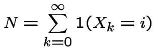


For last example: ![]() and
and ![]() are transient. Claim:
states 1, 2 and 3 are recurrent.
are transient. Claim:
states 1, 2 and 3 are recurrent.
Proof: argument above shows each transient state is visited only finitely many times. So: there is a recurrent state. (Note use of finite number of states.) It must be one of 1, 2 and 3. Proposition: If one state in a communicating class is recurrent then all states in the communicating class are recurrent.
Proof: Let ![]() be the known recurrent state so
be the known recurrent state so


Proposition also means that if 1 state in a class is transient so are all.
State ![]() has period
has period ![]() if
if ![]() is greatest common
divisor of
is greatest common
divisor of

 then
then
![$\displaystyle {\bf P}= \left[\begin{array}{ccccc}
0& 1 & 0 & 0 &0
\\
0 & 0 & ...
...0 & 0 & 0 & 0
\\
0 & 0 & 0 & 0 & 1
\\
0 & 0 & 0 & 1 & 0
\end{array}\right]
$](img399.gif)
 is a class of period 3 states
and
  a class of period 2 states.
![$\displaystyle {\bf P}= \left[\begin{array}{ccc}
0& 1/2 & 1/2
\\
1 & 0 & 0
\\
1 & 0 & 0
\end{array}\right]
$](img402.gif)
A chain is aperiodic if all its states are aperiodic.
Example: consider a sequence of independent coin tosses with probability ![]() of Heads on a single toss. Let
of Heads on a single toss. Let  be number of heads minus number of tails
after
 ![]() tosses. Put
tosses. Put  .
.
 is a Markov Chain. State space is
![]() , the integers and
, the integers and
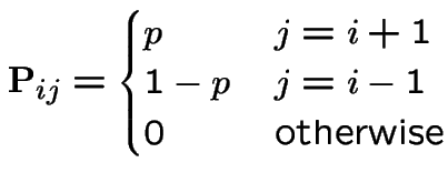
This chain has one communicating class (for  ) and
all states have period 2. According to the strong law of large
numbers
  converges to
  . If
. If  this guarantees
that for all large enough
 ![]()
 , that is, the number
of returns to 0 is not infinite. The state 0 is then transient
and so all states must be transient.
For  the situation is different. It is a fact that
 # H = # T at time $n$
 heads
in
Local Central Limit Theorem (normal approximation to
 ) (or Stirling's approximation) shows
 Binomial

Start irreducible recurrent chain  in state
 ![]() .
Let
.
Let ![]() be first
be first  such that
  .
Define

 |
 |
|
 |
||
 |
||
 |
Example
![$\displaystyle {\bf P}= \left[\begin{array}{cc} \frac{3}{5} & \frac{2}{5}
\\
\\
\frac{1}{5} & \frac{4}{5}
\end{array} \right]
$](img241.gif)
 |
 |
|
 |
 |
|
 |
 |
|
 |
 |
 |
 |
|
 |
 |
 |
 |
|
 |
 |
Notice stationary initial distribution is
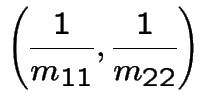


Heuristic: start chain in ![]() . Expect to return to
. Expect to return to ![]() every
every
 time units. So are in state
 ![]() about once every
about once every
 time units; i.e. limiting fraction of time in state
 ![]() is
is  .
.
Conclusion: for an irreducible recurrent finite state space Markov chain

Previous conclusion is still right if there is a stationary initial distribution.
Example:
 Heads
Heads![]() Tails after
Tails after ![]() tosses
of fair coin. Equations are
tosses
of fair coin. Equations are
 |
 |
|
 |
 |
Some observations:
You have to go through 1 to get to 0 from 2 so

Symmetry (switching H and T):

The transition probabilities are homogeneous:

Conclusion:
 |
 |
|
 |
||
 |
Summary of the situation:
Every state is recurrent.
All the expected hitting times  are infinite.
All entries
 converge to 0.
Jargon: The states in this chain are null recurrent.
Page 229, question 21: runner goes from front or back
door, prob 1/2 each. Returns front or back, prob 1/2 each.
Has ![]() pairs of shoes, wears pair if any at departure door,
leaves at return door. No shoes? Barefoot. Long run fraction
of time barefoot?
pairs of shoes, wears pair if any at departure door,
leaves at return door. No shoes? Barefoot. Long run fraction
of time barefoot?
Solution: Let  be number of shoes at front door on day
 ![]() .
Then
.
Then  is a Markov Chain.
Transition probabilities:
![]() pairs at front door on day
pairs at front door on day ![]() .
.  is
is ![]() if
goes out back door (prob is 1/2) or out front door and back
in front door (prob is 1/4). Otherwise
if
goes out back door (prob is 1/2) or out front door and back
in front door (prob is 1/4). Otherwise  is
is  .
.
 pairs at front door on day
 ![]() .
.  is
is  if out back, in front (prob is 1/4).
  is
is  if out
front, in back. Otherwise
  is
is ![]() .
.
0 pairs at front door on day ![]() .
.  is 0 if
out front door (prob 1/2) or out back door and in back door
(prob 1/4) otherwise
  is
is ![]() .
.
Transition matrix ![]() :
:
![$\displaystyle \left[\begin{array}{cccccc}
\frac{3}{4} & \frac{1}{4} & 0 & 0 &\c...
... \vdots
\\
0 & 0 & 0 & \cdots & \frac{1}{4} & \frac{3}{4}
\end{array}\right]
$](img468.gif)
Doubly stochastic: row sums and column sums are 1.
So
 for all
 ![]() is stationary initial distribution.
is stationary initial distribution.
Solution to problem: 1 day in  no shoes at front door. Half of
those go barefoot. Also 1 day in
  all shoes at front door; go
barefoot half of these days. Overall go barefoot
  of the time.
Insurance company's reserves fluctuate: sometimes up, sometimes down.
Ruin is event they hit 0 (company goes bankrupt). General problem.
For given model of fluctuation compute probability of ruin either
eventually or in next ![]() time units.
time units.
Simplest model: gambling on Red at Casino. Bet $1 at a time. Win
$1 with probability ![]() , lose $1 with probability
, lose $1 with probability  . Start with
![]() dollars. Quit playing
when down to $0 or up to
dollars. Quit playing
when down to $0 or up to ![]() . Compute
. Compute
 reach $N$ before $0$
 = fortune after
 ![]() plays.
plays.  .
.
Transition matrix:
![$\displaystyle {\bf P}=
\left[\begin{array}{cccccc}
1 & 0 & 0 & 0 &\cdots & 0
\...
... & \ddots & \ddots & \vdots
\\
0 & 0 & 0 & \cdots & 0 & 1
\end{array}\right]
$](img476.gif)
 |
||
 |
||
 |
 |
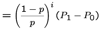
Middle equation is

 |
 |
|
 |
||
 |
||
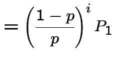 |
 to get
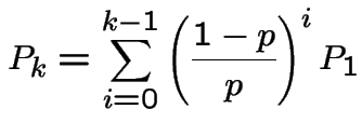

For ![]() we get
we get


Notice that if  our formulas for the sum of the geometric series
are wrong. But for
  we get

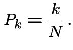
![$\displaystyle {\bf P}= \left[\begin{array}{cccc}
\frac{1}{2} & \frac{1}{2} & 0 ...
...\\
\frac{1}{4} & \frac{1}{4} & \frac{3}{8} & \frac{1}{8}
\end{array}\right]
$](img499.gif)
 be the expected
total number of visits to state
For ![]() or
or ![]() and
and  or 4:
or 4:

For  or
or 

For
 first step analysis:
 |
 |
|
 |
 |
|
 |
 |
|
 |
 |
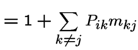
In matrix form
![$\displaystyle \left[\begin{array}{cc} m_{3,3} &m_{3,4} \\ \\ m_{4,3} &m_{4,4}\end{array}\right]$](img517.gif) |
![$\displaystyle = \left[\begin{array}{cc} 1 & 0 \\ \\ 0 & 1 \end{array}\right] +$](img518.gif) |
|
![$\displaystyle \qquad \left[\begin{array}{cc} \frac{1}{4} & \frac{1}{4} \\ \\ \f...
...eft[\begin{array}{cc} m_{3,3} &m_{3,4} \\ \\ m_{4,3} &m_{4,4}\end{array}\right]$](img519.gif) |
Translate to matrix notation:

 the
part of the transition matrix corresponding to transient states.
Solution is

![$\displaystyle {\bf I} - {\bf P}_T =
\left[\begin{array}{rr} \frac{3}{4} & -\frac{1}{4} \\ \\
-\frac{3}{8} & \frac{7}{8}
\end{array}\right]
$](img525.gif)
![$\displaystyle {\bf M} = \left[\begin{array}{rr} \frac{14}{9} & \frac{4}{9} \\ \\
\frac{2}{3} & \frac{4}{3}
\end{array}\right]
$](img526.gif)
Particles arriving over time at a particle detector. Several ways to describe most common model.
Approach 1: numbers of particles arriving in an interval has Poisson distribution, mean proportional to length of interval, numbers in several non-overlapping intervals independent.
For  , denote number of arrivals in
 ![$ (s,t]$](img528.gif) by
by  . Model is
 has a Poisson
 distribution.
 the variables
 are independent.
Approach 2:
Let
 be the times at which the particles
arrive.
Let
 with
with  by convention.
Then
 are independent Exponential random variables with mean
  .
.
Note
 is called survival function of
 ![]() .
.
Approaches are equivalent. Both are deductions of a model based on local behaviour of process.
Approach 3: Assume:
![$ [0,t]$](img540.gif) the probability of 1 point in the
interval
the probability of 1 point in the
interval ![$ (t,t+h]$](img541.gif) is of the form
is of the form

![$ [0,t]$](img540.gif) the probability of 2 or more points in
interval
the probability of 2 or more points in
interval ![$ (t,t+h]$](img541.gif) is of the form
is of the form

All 3 approaches are equivalent. I show: 3 implies 1, 1 implies 2
and 2 implies 3. First explain ![]() ,
, ![]() .
.
Notation: given functions ![]() and
and ![]() we write
we write


[Aside: if there is a constant ![]() such that
such that


 and
and 

 is tiny compared to
  is (very) roughly the same size as
Model 3 implies 1:
Fix ![]() , define
, define  to be conditional probability of 0 points in
![$ (t,t+s]$](img559.gif) given value of process on
given value of process on ![$ [0,t]$](img540.gif) .
.
Derive differential equation for
![]() . Given process on
. Given process on ![$ [0,t]$](img540.gif) and 0 points in
and 0 points in ![$ (t,t+s]$](img559.gif) probability of no
points in
probability of no
points in ![$ (t,t+s+h]$](img560.gif) is
is

![$ [0,t]$](img540.gif) the probability of no points in
the probability of no points in ![$ (t,t+s]$](img559.gif) is
is
 . Using
 gives
gives
 |
 |
|
 |

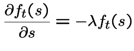

Notice: survival function of exponential rv..
General case. Notation:
 .
.
 is a non-decreasing function of
 ![]() . Let
. Let

 by conditioning on
 and
and  .
.
Given  probability that
 is conditional
probability of
  points in
 ![$ (t,t+h]$](img541.gif) .
.
So, for  :
:

 we have

 we have

![]() is increasing so only consider
is increasing so only consider  .
.
 |
 |
|
 |

 is dropped and

 we get


With  we get

 and
and


 has Poisson
 distribution.
Similar ideas permit proof of

If ![]() is a Poisson Process we define
is a Poisson Process we define
 to be the times between 0 and the first point, the first point and
the second and so on.
Fact:
 are iid exponential rvs with
mean
  .
.
We already did ![]() rigorously. The event
rigorously. The event  is exactly the
event
  . So
. So

I do case of  . Let
. Let  be two positive numbers and
 ,
,
 . Consider event

This is almost the same as the intersection of the four events:
![$\displaystyle N(0,t_1]$](img614.gif) |
 |
|
![$\displaystyle N(t_1,t_1+\delta_1]$](img615.gif) |
 |
|
![$\displaystyle N(t_1+\delta_1,t_1+\delta_1+t_2]$](img616.gif) |
 |
|
![$\displaystyle N(s_2+\delta_1,s_2+\delta_1+\delta_2]$](img617.gif) |
 |

 and let
  is
is

More rigor:
 .
.
 .
.
First step: Compute

![$ (s_{i-1},s_i]$](img626.gif) for
for
 (
( ) and at least one point in
![$ (s_{k-1},s_k]$](img629.gif) which has probability
which has probability

Second step: write this in terms of joint cdf of
 .
I do
 ![]() :
:

 .
.
Differentiate twice, that is, take
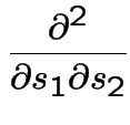


That completes the first part.
Now compute the joint cdf of  by
by

 |
 |
|
 |
||
 |
||
 |

Summary so far:
Have shown:
Instantaneous rates model implies independent Poisson increments model implies independent exponential interarrivals.
Next: show independent exponential interarrivals implies the instantaneous rates model.
Suppose
 iid exponential rvs with means
  . Define
![]() by
by  if and only if

Let ![]() be the event
be the event
 . We
are to show
![$\displaystyle P(N(t,t+h] = 1\vert N(t)=k,A) = \lambda h + o(h)
$](img650.gif)
![$\displaystyle P(N(t,t+h] \ge 2\vert N(t)=k,A) = o(h)
$](img651.gif)
If  is a possible trajectory consistent with
  then
then ![]() has jumps at points
has jumps at points

![$ (0,t]$](img655.gif) .
.
So given
 with
with  we are essentially being given


 irrelevant (independence).
![$\displaystyle P(N(t,t+h] = 1\vert$](img659.gif) |
 |
|
 |
||
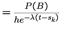 |

![$\displaystyle P
(N(t,t+h] = 1\vert N(t)=k,A) /h \to \lambda
$](img664.gif)
The computation of
![$\displaystyle \lim_{h\to 0} P(N(t,t+h] \ge 2\vert N(t)=k,A) /h
$](img665.gif)
Convolution: If ![]() and
and ![]() independent rvs with
densities
independent rvs with
densities ![]() and
and ![]() respectively and
respectively and  then
then


If
 iid Exponential
 then
then
 has a Gamma
 distribution. Density
of
 ![]() is
is

 .
.
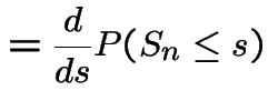
Proof:
 |
![$\displaystyle = P(N(0,s] < n)$](img677.gif) |
|
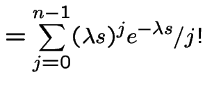 |
Then
 |
 |
|
 |
||
 |
||
 |
||
 |
||
 |

Extreme Values: If
 are independent exponential rvs
with means
 then
then
 has an exponential distribution with
mean

Proof:
 |
 |
|
 |
||
 |
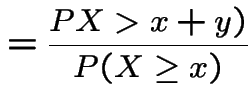
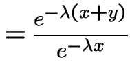
Memoryless Property: conditional distribution of
 given
given  is
exponential if
 ![]() has an exponential distribution.
has an exponential distribution.
Proof:
 |
||
 |
||
 |
||
 |
||
 |
The hazard rate, or instantaneous failure rate for a positive
random variable ![]() with density
with density ![]() and cdf
and cdf ![]() is
is

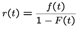
 this is
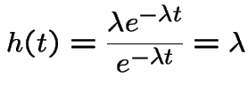
Weibull random variables have density

 . The corresponding survival function is


 , decreasing for
  . For
. For Since


 and
and  are independent Poisson processes with
rates
  is a Poisson process with rate
 .
.
 , independently of
all other occurences. Suppose
  ). Then
 are independent Poisson processes
with rates
 .
.
 independent rvs, each
uniformly distributed on
 ![$ [0,T]$](img731.gif) . Suppose
. Suppose  random variable independent of the
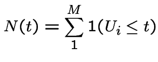
![$ [0,T]$](img731.gif) with rate
with rate  be the times at which points arrive
Given
 have the same distribution
as the order statistics of a sample of size
 ![$ [0,T]$](img731.gif) .
.
 ,
,
 have the same distribution
as the order statistics of a sample of size
 ![$ [0,T]$](img731.gif) .
.
Indications of some proofs:
1)
 independent Poisson processes rates
 ![]() ,
,
 . Let
. Let  be the event of 2 or more points
in
 ![]() in the time interval
in the time interval ![$ (t,t+h]$](img541.gif) ,
,  , the event of exactly
one point in
 ![]() in the time interval
in the time interval ![$ (t,t+h]$](img541.gif) .
.
Let  and
and  be the corresponding events for
 ![]() .
.
Let ![]() denote the history of the processes up to time
denote the history of the processes up to time ![]() ; we
condition on
; we
condition on ![]() .
.
We are given:


Note that

Since
 |
 |
|
 |
||
 |
||
 |
Next let ![]() be the event of no points in
be the event of no points in
![]() in the time interval
in the time interval ![$ (t,t+h]$](img541.gif) and
and  the same
for
 ![]() .
Then
.
Then
 |
 |
|
 |
||
 |
||
 |
 |
 |
|
 |
 .
.
2) The infinitesimal approach used for 1 can do part of this.
See text for rest. Events defined as in 1):
The event  that there is one point in
 ![]() in
in ![$ (t,t+h]$](img541.gif) is the event,
is the event,
 that there is exactly one point in any of the
 ![]() processes together
with a subset of
processes together
with a subset of  where there are two or more points in
 ![]() in
in
![$ (t,t+h]$](img541.gif) but exactly one is labeled
but exactly one is labeled ![]() . Since
. Since

 |
 |
|
 |
||
 |
Similarly,  is a subset of
  so
so

 . To
get independence requires more work; see the text for the algebraic
method which is easier.
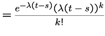
3) Fix  . Let
. Let  be the number of points
in
 ![$ (s,t]$](img528.gif) . Given
. Given ![]() the conditional distribution of
the conditional distribution of
 is Binomial
 with
with
 . So
. So
 |
 |
|
 |
||
 |
||
 |
||
 |
||
 |
||
 |
||
 |
4): Fix  for
for
 such that

 we compute the probability of the event

 is (
is ( ):
):
![\begin{multline*}
B \equiv \\
\bigcap_{i=1}^n \{N(s_{i-1}+h_{i-1},s_i]=0,N(s_i,s_i+h_i]=1\}
\\
\cap \{N(s_n+h_n,T]=0\}
\end{multline*}](img787.gif)

 |
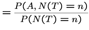 |
|
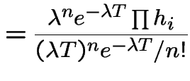 |
||
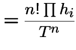 |
Divide by  and let all
 ![]() go to 0 to
get joint density of
go to 0 to
get joint density of
 is
is

![$ [0,T]$](img731.gif) sample
of size
sample
of size
5) Replace the event  with
with
 . With
![]() as before we want
as before we want
![\begin{multline*}
P(A\vert T < S_{n+1}< T+h)
\\
= \frac{ P(B,N(T,T+h] \ge 1)}{P(T < S_{n+1}< T+h)}
\end{multline*}](img797.gif)
![$ \{N(T,T+h] \ge 1\}$](img798.gif) and that we have
already found the limit
and that we have
already found the limit
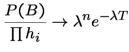
We are left to compute the limit of
![$\displaystyle \frac{P(N(T,T+h] \ge 1)}{P(T < S_{n+1}< T+h)}
$](img800.gif)
![\begin{multline*}
\sum_{k=0}^n P(N(0,T]=k,N(T,T+h]=n+1-k)
\\
+o(h) = P(N(0,T]=n)\lambda h+o(h)
\end{multline*}](img801.gif)
![$\displaystyle \frac{P(N(T,T+h] \ge 1)}{P(T < S_{n+1}< T+h)}
$](img800.gif) |
 |
|
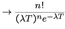 |
 given
given  as in 4).
The idea of hazard rate can be used to extend the notion of Poisson
Process. Suppose
 is a function of
 ![]() . Suppose
. Suppose
![]() is a counting process such that
is a counting process such that


 has a Poisson distribution with mean
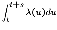
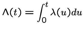
 is
is
 .
.
Jargon: ![]() is the intensity or instaneous intensity
and
is the intensity or instaneous intensity
and ![]() the cumulative intensity.
the cumulative intensity.
Can use the model with ![]() any non-decreasing right continuous
function, possibly without a derivative. This allows ties.
any non-decreasing right continuous
function, possibly without a derivative. This allows ties.
Imagine insurance claims arise at times of a Poisson process,  ,
(more likely for an inhomogeneous process).
Let ![]() be the value of the
be the value of the ![]() th claim associated
with the point whose time is
th claim associated
with the point whose time is ![]() .
.
Assume that the ![]() 's are independent of each other and of
's are independent of each other and of
![]() .
.
Let
 and
and 
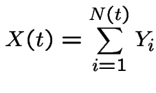
Useful properties:
 |
 |
|
 |
 |
|
 |
 |
|
 |
||
 |
![$\displaystyle = {\rm Var}\left[{\rm E}\left\{X(t)\vert N(t)\right\}\right]$](img825.gif) |
|
![$\displaystyle \qquad +{\rm E}\left[{\rm Var}\left\{X(t)\vert N(t)\right\}\right]$](img826.gif) |
||
 |
Consider a population of single celled organisms in a stable environment.
Fix short time interval, length ![]() .
.
Each organism has some probability of dividing to produce two organisms and some other probability of dying.
We might suppose:
 .
.
 .
.
 .
.
Tacit assumptions:
Constants of proportionality do not depend on time: ``stable environment''.
Constants do not depend on organism: organisms are all similar and live in similar environments.
 : total population at time
 ![]() .
.
![]() : history of
process up to time
: history of
process up to time ![]() .
.
Condition on event  .
.
Probability of two or more divisions
(more than one division by a single organism or two or more organisms dividing)
is  .
.
Probability of both a division and a death
or of two or more deaths is  .
.
So probability of exactly 1 division by any one of the ![]() organisms is
organisms is
 .
.
Similarly probability of 1 death is
 .
.
We deduce:
 |
 |
|
 |
||
 |
 |
|
 |
||
 |
 |
|
 |
||
 |
 |
|
 |
These equations lead to:
 |
 |
|
 |
||
 |
This is the Markov Property.
Definition:A process
 taking values in
![]() , a finite or countable state space is a Markov Chain
if
, a finite or countable state space is a Markov Chain
if
 |
 |
|
 |
||
 |
Definition:A Markov chain ![]() has stationary transitions if
has stationary transitions if

From now on: our chains have stationary transitions.

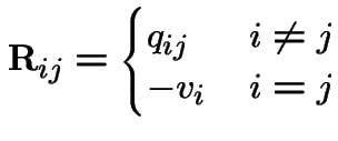
 is Markov chain - transition matrix has
 .
.


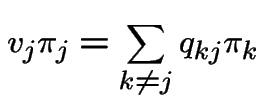

 if
if 


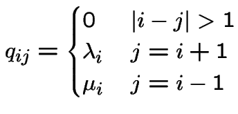
 then process is a pure birth process.
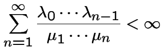
If all
 a pure death process.


 .
.
Suppose ![]() a Markov Chain with stationary transitions.
Then
a Markov Chain with stationary transitions.
Then
 |
 |
|
 |
||
 |
||
 |
||
 |
||
 |
||
 |
||
 |
This shows

Now consider the chain starting from ![]() and let
and let ![]() be
the first
be
the first ![]() for which
for which
 . Then
 ![]() is
a stopping time.
is
a stopping time.
[Technically:

 |
 |
|
 |
||
 |
Conclusion: given  ,
, ![]() has memoryless property
so
has memoryless property
so ![]() has an exponential distribution. Let
has an exponential distribution. Let ![]() be the
rate parameter.
be the
rate parameter.
Let
 be the stopping times at which
transitions occur. Then
 . The sequence
  is a Markov chain by the
Markov property. That
 reflects the fact
that
 by design.
As before we say
 if
if
 for some
 ![]() .
It is fairly clear that
.
It is fairly clear that
 for the
  if and only
if
 for the embedded chain
  .
.
We say
 (
(![]() and
and ![]() communicate) if
communicate) if
 and
and
 .
.
Now consider

 . Then the event
  is, except
for possibilities of probability
  the event that
 and
and 

The Chapman-Kolmogorov equations are

 from both sides, divide by
  is the identity.
We find


The Chapman-Kolmogorov equations can also be written

 from both sides, dividing by
Look at these equations in component form:


 our calculations of instantaneous transition
rates gives


 either means
  which has probability
![$ [0,h]$](img920.gif) , a possibility of probability
, a possibility of probability  .)
Thus

Let ![]() be the matrix with entries
be the matrix with entries


![]() is the infinitesimal generator of the chain.
is the infinitesimal generator of the chain.
Thus

 |
 |
|
 |
On the other hand

 |
 |
|
 |
Remark: When the state space is infinite the forward equations may not be justified. In deriving them we interchanged a limit with an infinite sum; the interchange is always justified for the backward equations but not for forward.
Example:  . Then
![$\displaystyle {\bf P}= \left[\begin{array}{cc} 0 & 1 \\ 1 & 0 \end{array}\right]
$](img931.gif)
![$\displaystyle {\bf R}= \left[\begin{array}{cc}-v_0 & v_0 \\ v_1 & -v_1 \end{array}\right]
$](img934.gif)
 |
 |
|
 |
 |
|
 |
 |
|
 |
 |
 |
 |
|
 |
 |
|
 |
 |
|
 |
 |
Add  first plus
  third backward equations to get


 . This gives


Alternative calculation:
![$\displaystyle {\bf R}= \left[\begin{array}{cc}-v_0 & v_0 \\ v_1 & -v_1 \end{array}\right]
$](img934.gif)

![$\displaystyle {\bf M} = \left[\begin{array}{cc} 1 & v_0\\ \\ 1 & -v_1\end{array}\right]
$](img959.gif)
![$\displaystyle {\bf M}^{-1} = \left[\begin{array}{cc} \frac{v_1}{v_0+v_1} & \frac{v_0}{v_0+v_1}
\\ \\ \frac{1}{v_0+v_1} & \frac{-1}{v_0+v_1}\end{array}\right]
$](img960.gif)
![$\displaystyle {\bf\Lambda} = \left[\begin{array}{cc} 0 & 0\\ \\ 0 & -(v_0+v_1)\end{array}\right]
$](img961.gif)
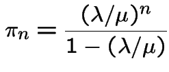
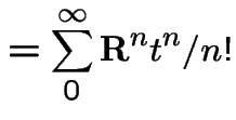
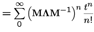
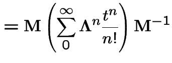
Then
 |
 |
|
 |
||
 |
![$\displaystyle \sum_0^\infty{\bf\Lambda}^n\frac{t^n}{n!} = \left[\begin{array}{cc}1 & 0 \\ 0&
e^{-(v_0+v_1)t}\end{array}\right]
$](img966.gif)
 |
 |
|
![$\displaystyle = {\bf M} \left[\begin{array}{cc}1 & 0 \\ 0& e^{-(v_0+v_1)t}\end{array}\right]{\bf M}^{-1}$](img969.gif) |
||
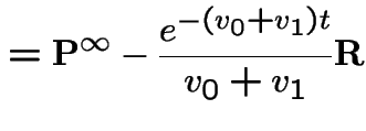 |
![$\displaystyle {\bf P}^\infty=\left[\begin{array}{cc} \frac{v_1}{v_0+v_1} & \fra...
..._0+v_1}
\\
\\
\frac{v_1}{v_0+v_1} & \frac{v_0}{v_0+v_1}
\end{array}\right]
$](img971.gif)
Notice: rows of
![]() are a stationary initial distribution. If rows are
are a stationary initial distribution. If rows are
![]() then
then
![$\displaystyle {\bf P}^\infty = \left[\begin{array}{c}1 \\ 1 \end{array}\right] \pi \equiv {\bf 1}\pi
$](img972.gif)


Fact:
 is long run fraction of time in
state 0.
Fact:

Consider a population of  individuals. Suppose
in next time interval
  probability of population
increase of 1 (called a birth) is
 and
probability of decrease of 1 (death) is
 .
.
Jargon: ![]() is a birth and death process.
is a birth and death process.
Special cases:
All  ; called a pure birth process.
All
 (0 is absorbing): pure death process.
 and
and
 is a linear
birth and death process.
 ,
,
 : Poisson Process.
 and
and
 is a linear
birth and death process with immigration.
Ingredients of Queuing Problem:
1: Queue input process.
2: Number of servers
3: Queue discipline: first come first serve? last in first out? pre-emptive priorities?
4: Service time distribution.
Example:
Imagine customers arriving at a facility at times of a Poisson
Process ![]() with rate
with rate ![]() . This is the input process,
denoted
. This is the input process,
denoted ![]() (for Markov) in queuing literature.
(for Markov) in queuing literature.
Single server case:
Service distribution: exponential service times, rate ![]() .
.
Queue discipline: first come first serve.
 = number of customers in line at time
 ![]() .
.
![]() is a Markov process called
is a Markov process called  queue:

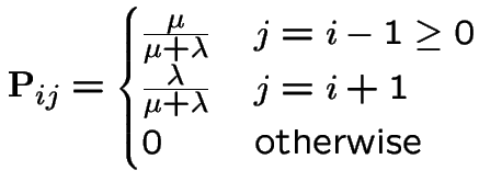
Example:
 queue:
Customers arrive according to PP rate ![]() . Each
customer begins service immediately.
. Each
customer begins service immediately.  is number
being served at time
 ![]() .
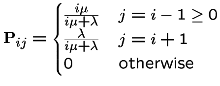
. ![]() is a birth and death process
with
is a birth and death process
with

We have seen that a stationary initial distribution ![]() is
a probability vector solving
is
a probability vector solving

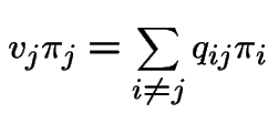

So equation says:
Rate of departure from ![]() balances rate of arrival to
balances rate of arrival to ![]() . This is called
balance.
. This is called
balance.
Application to birth and death processes:
Equation is

 and
and

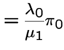 |
||
 |
||
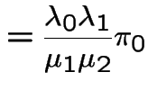 |

Apply
 to get


If


 is constant. Put
For fair random walk ![]() = number of heads minus number of
tails,
= number of heads minus number of
tails,


 |
 |
|
 |
 |

 .
.
We now turn these pictures into a stochastic process:
For
 we define


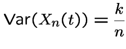
 . Moreover:

 by the central limit theorem. Thus

Another observation:
 is independent of
  because the
two rvs involve sums of different
 ![]() .
.
Conclusions.
As
![]() the processes
the processes  converge to a process
![]() with the properties:
with the properties:
 has a
has a  distribution.


 .
.
Definition:Any process satisfying 1-4 above is a Brownian motion.
 . Then
 |
 |
|
 |
||
 |
||
 |
 .
.
 :
:
 |
 |
|
 |
||
 |
||
 |
||
 |
Suppose  . Then
 is a sum
of two independent normal variables. Do following calculation:
 , and
, and
 independent.
  .
.
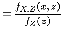
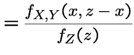
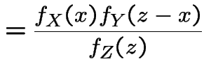
Compute conditional distribution of ![]() given
given ![]() :
:
 |
 |
|
 |
||
 |
 where
where
 so
so
 |
 |
|
 |
Coefficient of ![]() :
:

 .
.
Coefficient of ![]() :
:


Finally you should check that
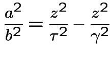
Conclusion: given ![]() the conditional distribution of
the conditional distribution of ![]() is
is
 with
with ![]() and
and ![]() as above.
as above.
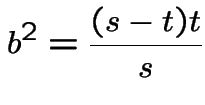
Application to Brownian motion:
 let
let  and
and  so
so
 . Then
 and
and
 .
Thus


Tossing a fair coin:
| HTHHHTHTHHTHHHTTHTH | 5 more heads than tails |
| THTTTHTHTTHTTTHHTHT | 5 more tails than heads |
Both sequences have the same probability.
So: for random walk starting at stopping time:
Any sequence with ![]() more heads than tails in
next
more heads than tails in
next ![]() tosses is matched to sequence with
tosses is matched to sequence with ![]() more
tails than heads. Both sequences have same prob.
more
tails than heads. Both sequences have same prob.
Suppose ![]() is a fair (
is a fair ( ) random walk. Define

Compute
 ?
Trick: Compute

First: if  then
then

Second: if  then
then

Fix  . Consider a sequence of H's and T's which leads
to say
 ![]() and
and  .
.
Switch the results of tosses
 to
to ![]() to get a sequence of H's and T's which
has
to get a sequence of H's and T's which
has ![]() and
and
 . This proves

This is true for each ![]() so
so
 |
 |
|
 |
Finally, sum over all ![]() to get
to get
 |
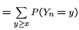 |
|
 |
Make the substitution  in the second sum to get
 |
 |
|
 |
||
 |
Brownian motion version:


Any path with  and
and  is matched
to an equally likely path with
 and
and
 .
.
So for 


Let  to get
 |
 |
|
 |
 |
 |
|
 |
 has the distribution
of
  .
.
On the other hand in view of


 is 1 minus the standard normal
cdf.
So
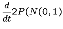 |
 |
|
 |
||
 |
NOTE: the preceding is a density when viewed as
a function of the variable ![]() .
.
A stochastic process  indexed by either a
discrete or continuous time parameter
 ![]() is a
martingale if:
is a
martingale if:

 .
.
Examples
 is a Poisson Process with rate
  is a martingale.
Note: Brownian motion with drift is a process of the form

 . We call
 is a Brownian motion with drift then

 a martingale.
 is the amount of money s/he has after
  is
a martingale - even if the bets made depend on the outcomes of
previous bets, that is, even if the gambler plays a strategy.
Some evidence for some of the above:
Random walk:
 iid with

 with
with  . Then
 |
 |
|
 |
||
 |
||
 |
||
 |
||
 |
![]() treated as constant given
treated as constant given
 .
.
Knowing
 is equivalent to knowing
 .
.
For  we have
 ![]() independent of
independent of
 so conditional expectation is unconditional expectation.
Since Standard Brownian Motion is limit of such random walks we get martingale property for standard Brownian motion.
Poisson Process:
 . Fix
. Fix  .
.
 |
 |
|
 |
||
 |
||
 |
||
 |
||
 |
||
 |
Things to notice:
I used independent increments.
 is shorthand for the conditioning event.
Similar to random walk calculation.
We model the price of a stock as


If annual interest rates are
 we call
 ![]() the
instantaneous interest rate; if we invest $1 at time 0 then
at time
the
instantaneous interest rate; if we invest $1 at time 0 then
at time ![]() we would have
we would have
![]() . In this sense
an amount of money
. In this sense
an amount of money  to be paid at time
 ![]() is worth
only
is worth
only
 at time 0 (because that much money at
time 0 will grow to
  by time
 ![]() ).
).
Present Value: If the stock price at time ![]() is
is  per share
then the present value of 1 share to be delivered at time
 ![]() is
is


Now we compute

 . Write

![\begin{multline*}
{\rm E}\left\{ Z(t) \vert B(u);0 \le u \le s\right\}
\\
= x_...
...\mu-\alpha)t} \times
{\rm E}\left[e^{\sigma\{B(t)-B(s)\}}\right]
\end{multline*}](img1168.gif)
Note:  is
is  ; the expected
value needed is the moment generating function of this variable at
![]() .
.
Suppose
 . The Moment Generating Function of
 ![]() is
is

Rewrite

 to see
![$\displaystyle {\rm E}\left[e^{\sigma\{B(t)-B(s)\}}\right]= e^{\sigma^2(t-s)/2}
$](img1174.gif)
 |
 |
|
 |
||
 |

If this identity is satisfied then the present value of the stock price is a martingale.
Suppose you can pay $![]() today for the right to pay
today for the right to pay ![]() for
a share of this stock at time
for
a share of this stock at time ![]() (regardless of the actual price
at time
(regardless of the actual price
at time ![]() ).
).
If, at time ![]() ,
,  you will exercise your option
and buy the share making
  dollars.
If
 you will not exercise your option; it becomes
worthless.
The present value of this option is

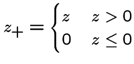
In a fair market:
 is a martingale.
So:
![$\displaystyle c = {\rm E}\left[ e^{-\alpha t}\left\{X(t) - K\right\}_+\right]
$](img1187.gif)
Since


This is

 |
||
 |
||
 |
Evidently

The other integral needed is
 |
 |
|
 |
||
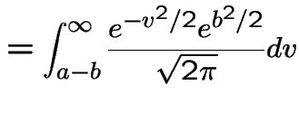 |
||
 |
Introduce the notation

 |
||
 |
||
 |
This is the Black-Scholes option pricing formula.
Monte Carlo computation of expected value:
To compute
 : do experiment
 ![]() times to generate
times to generate
![]() independent observations all with same distribution as
independent observations all with same distribution as
![]() .
.
Get
 .
.
Use
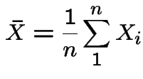

To estimate
 : use same
 ![]() and compute
and compute
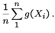
In practice: random quantities are not used.
Use: pseudo-random uniform random numbers.
They ``behave like'' iid Uniform(0,1) variables.
Many, many generators. One standard kind: linear congruential generators.
Start with ![]() an integer in range
an integer in range
 .
Compute

Integers ![]() and
and ![]() are chosen so that
are chosen so that
 runs through the set
 (or as much of it is possible, sometimes).

 .
.
 .
.
Use

We now pretend we can generate
 which are iid Uniform(0,1).
Monte Carlo methods for generating a sample:
Fact: ![]() continuous CDF and
continuous CDF and  satisfy

Proof: For simplicity: assume ![]() strictly increasing on
inverval
strictly increasing on
inverval  with
with  and
and  .
.
If ![]() Uniform(0,1) then
Uniform(0,1) then
 |
 |
|
 |
||
 |
Conversely: if ![]() and
and  then
there is a unique
 ![]() such that
such that 
 |
 |
|
 |
||
 |
||
 |
Application: generate ![]() and solve
and solve  for
for ![]() to get
to get
 which has cdf
 ![]() .
.
Example:For the exponential distribution

 and solve to get

Observation:
 so
so
 also has
an Exponential(
also has
an Exponential(![]() ) distribution.
) distribution.
Example:: for ![]() the standard normal cdf solving
the standard normal cdf solving

Special purpose transformations:
Example:: If ![]() and
and ![]() are iid
are iid  define
 and
and
 by
by

NOTE: Book says

 ; notation

 so that

Then

 and go clockwise
to angle
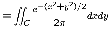
Compute joint cdf of  at
at
 .
.
Define

 |
 |
|
 |
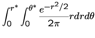


So

Moreover
![]() has cdf
has cdf

 .
.
![]() is Uniform
is Uniform .
.
So: generate  iid Uniform(0,1).
Define


You have generated two independent  variables.
If  difficult to solve (eg
 ![]() hard
to compute) sometimes use acceptance rejection.
hard
to compute) sometimes use acceptance rejection.
Goal: generate ![]() where
where
 .
.
Tactic: find density ![]() and constant
and constant ![]() such that
such that

Algorithm:
 let
let
Facts:
 |
![$\displaystyle \le f(Y)/\{cg(Y)\}]$](img1281.gif) |
|
![$\displaystyle = \int P[U \le f(y)/\{cg(y)\}\vert Y=y]g(y) dy$](img1282.gif) |
||
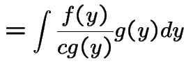 |
||
 |
||
 |

Most important fact:  :
:
Proof: this is like the old craps example:
We compute
![$\displaystyle P( X \le x) = P[ Y \le x\vert U \le f(Y)/\{cg(Y)\}]
$](img1288.gif)
Condition on ![]() to get
to get
 |
 |
|
![$\displaystyle = \frac{\int_{-\infty}^x P[U \le f(Y)/\{cg(Y)\}\vert Y=y]g(y)dy}{ P[U \le f(Y)/\{cg(Y)\}]}$](img1290.gif) |
||
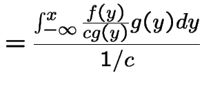 |
||
 |
||
 |
Example:Half normal distribution: ![]() has density
has density

 .)
.)
Use
 . To find
 ![]() maximize
maximize

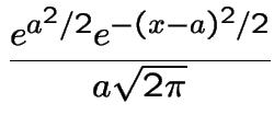
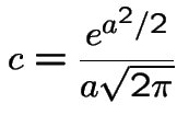
Choose ![]() to minimize
to minimize ![]() (or
(or  ); get
![]() so
so

Algorithm is then: generate
 and
then compute


To generate  : use a third
 ![]() to pick a sign
at random: negative if
to pick a sign
at random: negative if  otherwise positive.
The inverse transformation method works for discrete distributions.
![]() has possible values
has possible values
 with
probabilities
 compute
cumulative probabilities

 .
.
Generate ![]() Uniform(0,1).
Uniform(0,1).
Find ![]() such that
such that

Put  .
.