Postscript version of this file

STAT 450

Linear Algebra Review Notes

Notation:

• Vectors $x\in R^n$ are column vectors
  
  $$x=\left[\begin{array}{c} x_1 \\ \vdots \\ x_n \end{array}\right]$$
  
  

• An $m \times n$ matrix A has m rows, n columns and entries A_ij.

• Matrix and vector addition are defined componentwise:
  
  $$(A+B)_{ij} = A_{ij} +B_{ij} ; \qquad (x+y)_i = x_i + y_i$$
  
  

• If A is $m \times n$ and B is $n \times r$ then AB is the $m \times r$ matrix
  
  $$(AB)_{ij} = \sum_{k=1}^n A_{ik} B_{kj}$$
  
  

• The matrix I or sometimes $I_{n \times n}$ which is an $n \times n$matrix with I_ii = 1 for all i and I_ij=0 for any pair $i \neq j$ is called the $n \times n$ identity matrix.

• The span of a set of vectors $\{ x_1,\ldots,x_p\}$ is the set of all vectors x of the form $x=\sum c_i x_i$. It is a vector space. The column space of a matrix, A, is the span of the set of columns of A. The row space is the span of the set of rows.

• A set of vectors $\{ x_1,\ldots,x_p\}$ is linearly independent if $\sum c_i x_i = 0$ implies c_i=0 for all i. The dimension of a vector space is the cardinality of the largest possible set of linearly independent vectors.

Definition: The transpose, A^T, of an $m \times n$ matrix A is the $n \times m$ matrix whose entries are given by

(A^T)_ij = A_ji

so that A^T is $n \times m$. We have

(A+B)^T = A^T+B^T

and

$$(AB)^T = B^T A^T \, .$$

Definition: The rank of a matrix A is the number of linear independent columns of A; we use $\text{rank}(A)$ for notation. We have
$$\begin{align*}\text{rank}(A) & = \text{dim}(\text{column space of $A$ }) \\ & = \text{dim}(\text{row space of $A$ }) \\ & = \text{rank}(A^T) \end{align*}$$

If A is $m \times n$ then $\text{rank}(A) \le \min(m,n)$.

Matrix inverses

For this little section all matrices are square $n \times n$ matrices.

If there is a matrix B such that $BA=I_{n \times n}$ then we call B the inverse of A. If B exists it is unique and AB=I and we write B=A^-1. The matrix A has an inverse if and only if $\text{rank}(A) = n$.

Inverses have the following properties:

(AB)^-1 = B^-1A^-1

(if one side exists then so does the other) and

(A^T)^-1 = (A^-1)^T

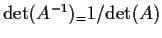
Determinants

Again A is $n \times n$. The determinant if a function on the set of $n \times n$ matrices such that:

1.

$\text{det}(I) = 1$.

2.

If $A^\prime$ is the matrix A with two columns interchanged then

$$\text{det}(A^\lq prime) = - \text{det}(A)\, .$$

(Notice that this means that two equal columns guarantees $\text{det}(A)=0$.)

3.

$\text{det}(A)$ is a linear function of each column of A. That is if $A = ( a_1, \ldots, a_n)$ with a_i denoting the ith column of the matrix then
$$\begin{align*}\text{det}(a_1,\ldots,a_i+b_i,\ldots,a_n) = & \text{det}(a_1,\ldots,a_i,\ldots,a_n) \\ & + \text{det}(a_1,\ldots,b_i,\ldots,a_n) \end{align*}$$

Here are some properties of the determinant:

4.

$\text{det}(A^T) = \text{det}(A)$.

5.

$\text{det}(AB) = \text{det}(A)\text{det}(B)$.

6.

$\text{det}(A^{-1})_ = 1/\text{det}(A)$.

7.

A is invertible if and only if $\text{det}(A) \neq 0$ if and only if $\text{rank}(A) = n$.

8.

Determinants can be computed (slowly) by expansion by minors.

Special Kinds of Matrices

1.

A is symmetric if A^T=A.

2.

A is orthogonal if A^T=A^-1 (or AA^T = A^TA=I).

3.

A is idempotent if $AA\equiv A^2 = A$.

4.

A is diagonal if $i \neq j$ implies A_ij=0.

Inner Products and orthogonal and orthonormal vectors

Definition: Two vectors x and y are orthogonal if $x^T y = \sum x_i y_i = 0$.

Definition: The inner product or dot product of x and y is

$$<x,y> = x^Ty = \sum x_i y_i$$

Definition: x and y are orthogonal if x^Ty=0.

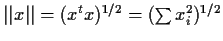
Definition: The norm (or length) of x is $\vert\vert x\vert\vert = (x^tx)^{1/2} = (\sum x_i^2)^{1/2}$

A is orthogonal if each column of A has length 1 and is orthogonal to each other column of A.

Quadratic Forms

Suppose A is an $n \times n$ matirx. The function

g(x) = x^T A x

is called a quadratic form. Now
$$\begin{align*}g(x) & = \sum_{ij} A_{ij} x_i x_j \\ & = \sum_i A_{ii} x_i^2 + \sum_{i < j} (A_{ij}+A_{ji}) x_ix_j \end{align*}$$
so that g(x) depends only on the total A_ij+A_ji. In fact

$$x^T Ax = x^T A^T x = x^T\left(\frac{A+A^T}{2} \right) x$$

Thus we will assume that A is symmetric.

Eigenvalues and eigenvectors

If A is $n \times n$ and $v\neq 0\in R^n$ and $\lambda\in R$ are such that

$$Av=\lambda v$$

then we saythat $\lambda$ is an eigenvalue (or characteristic value or latent value) of A and that v is the corresponding eigenvector. Since $Av-\lambda v = (A-\lambda I)v=0$ we find that $A-\lambda I$ must be singular. Therefore $\text{det}(A-\lambda I) =0$. Conversely if $A-\lambda I$ is singular then there is a $v \neq 0$ such that $(A-\lambda I)v=0$. In fact, $\text{det}(A-\lambda I)$ is a polynomial function of $\lambda$ of degree n. Each root is an eigenvalue. For general A the roots could be multiple roots or complex valued.

Diagonalization

A matrix A is diagonalized by a non-singular matrix P is $P^{-1} A P \equiv D$ is a diagonal matrix. If so then AP=PD and each column of P is an eignevector of A with the ith column having eigenvlaue D_ii. Thus to be diagonalizable A must have n linearly independent eigenvectors.

Symmetric Matrices

If A is symmetric then

1.

Every eigenvalue of A is real (not complex).

2.

A is diagonalizable and the columns of P may be taken to be orthogonal to each other and of unit length. In other words, A is diagonalizable by an orthogonal matrix P; in symbols P^TAP = D. The diagonal entries in D are the eigenvalues of A.

3.

If $\lambda_1 \neq \lambda_2$ are two eigenvalues of Aand v₁ and v₂ are corresponding eigenvectors then

$$v_1^T A v_2 = v_1^T \lambda_2 v_2 = \lambda_2 v_1^T v_2$$

and
$$\begin{align*}(v_1^T A v_2 )& = (v_1^T A v_2 )^T \\ & = v2^T A^T v_1 \\ & = v_2^T A v_1 \\ & = v_2^T \lambda_1 v_1 \\ & = \lambda_1 v_2^T v_1 \end{align*}$$
Since $(\lambda_1-\lambda_2)v_1^t v_2 =0$ and $\lambda_1 \neq \lambda_2$ we see that v₁^T v₂ = 0. In other words eigenvectors corresponding to distinct eigenvalues are orthogonal.

Orthogonal Projections

Suppose that S is a vector subspace of Rⁿ and that $a_1,\ldots,a_m$ are a basis for S. Given any $x\in R^n$ there is a unique $y\in S$ which is closest to x. That is, y minimizes

(x-y)^T(X-y)

over $y\in S$. Any y in S is of the form

$$y = c_1 a_1 + \cdots + c_m a_m = Ac$$

where A is the $n \times m$ matrix with columns $a_1,\ldots,a_m$ and c is the column vector with ith entry c_i. Define

Q= A(A^TA)^-1A^T

(The fact that A has rank m guarantees that A^TA is invertible.) Then
$$\begin{align*}(x-Ac)^T(x-Ac) & = (x-Qx+Qx-Ac)^T (x-Qx+Qx-Ac) \\ & = (x-Qx)^T(x-... ...+ (Qx-Ac)^T(x-Qx) \\ & \qquad +(x-Qx)^T(Qx-Ac) + (Qx-Ac)^T(Qx-Ac) \end{align*}$$
Note that x-Qx = (I-Q)x and that

QAc = A(A^TA)^-1A^TAc = Ac

so that

Qx-Ac = Q(x-Ac)

Then

(Qx-Ac)^T(x-Qx) = (x-Ac)^T Q^T (I-Q) x

Since Q^T=Q we see that
$$\begin{align*}Q^T(I-Q) & = Q(I-Q) \\ & = Q-Q^2 \\ & = Q-A(A^TA)^{-1}A^TA(A^TA)^{-1}A^T \\ & = Q-Q \\ & = 0 \end{align*}$$
This shows that

(x-Ac)^T(x-Ac) = (x-Qx)^T(x-Qx) + (Qx-Ac)^T(Qx-Ac)

Now to choose Ac to minimize this quantity we need only minimize the second term. This is achieved by making Qx=Ac. Since Qx=A(A^TA)^-1A^T x this can be done by taking c=(A^TA)^-1A^T x. In summary we find that the closest point y in S is

y=Qx=A(A^TA)^-1A^T x

We call y the orthogonal projection of x onto S.

Notice that the matrix Q is idempotent:

Q²=Q

We call Qx the orthogonal projection of x on S because Qx is perpendicular to the residual x-Qx=(I-Q)x.

Partitioned Matrices

Suppose that A₁₁ is a $p \times r$ matrix, A_1,2 is $p \times s$, A_2,1 is $q \times r$ and A_2,2 is $q \times s$. Then we could make a big $(p+q) \times (r+s)$ matrix by putting together the A_ij in a 2 by 2 matrix giving the following picture:

$$A = \left[ \begin{array}{cc} A_{11} & A_{12} \\ A_{21} & A_{22} \end{array}\right]$$

For instance if

$$A_{11} = \left[ \begin{array}{cc} 1 & 0 \\ 0 & 1 \end{array}\right]$$

$$A_{12} = \left[ \begin{array}{c} 2 \\ 3 \end{array}\right]$$

$$A_{21} = \left[ \begin{array}{cc} 4 & 5\end{array}\right]$$

and

$$A_{22} = \left[ 6 \right]$$

then

$$A = \left[ \begin{array}{cc\vert c} 1 & 0 & 2 \\ 0 & 1 & 3 \\ \hline 4 & 5 & 6 \end{array}\right]$$

where I have drawn in lines to indicate the partitioning.

We can work with partitioned matrices just like ordinary matrices always making sure that in products we never change the order of multiplication of things.

$$\left[ \begin{array}{cc} A_{11} & A_{12} \\ A_{21} & A_{22} ... ...2}+B_{12} \\ A_{21}+B_{21} & A_{22}+B_{22} \end{array}\right]$$

and

$$\left[ \begin{array}{cc} A_{11} & A_{12} \\ A_{21} & A_{22} ... ...1}+A_{22}B_{21} &A_{21}B_{12}+ A_{22}B_{22} \end{array}\right]$$

In these formulas the partitioning of A and B must match. For the addition formula the dimensions of A_ij and B_ijmust be the same. For the multiplication formula A₁₂ must have as many columns as B₂₁ has rows and so on. In general A_ij and B_jk must be of the right size for A_ijB_jkto make sense for each i,j,k.

The technique can be used with more than a 2 by 2 partitioning.

Definition: A block diagonal matrix is a partitioned matrix Awith pieces A_ij for which A_ij=0 if $i \neq j$. If

$$A = \left[ \begin{array}{cc} A_{11} & 0 \\ 0 & A_{22} \end{array}\right]$$

then A is invertible if and only if each A_ii is invertible and then

$$A^{-1} = \left[ \begin{array}{cc} A_{11}^{-1} & 0 \\ 0 & A_{22}^{-1} \end{array}\right]$$

Moreover $\text{det}(A) = \text{det}(A_{11}) \text{det}(A_{22})$. Similar formulas work for larger matrices.