Motivating examples:
1): Octopuses eaten by ling cod. Octopus beaks not digested; remain in cod stomach. Idea: make measurements on beaks to determine sex of eaten octopus -- to determine where the different sexes live.
2): Digitized scan of handwritten number: 32![]() 32
grid of pixels each either black or white.
From vector of 256 numbers determine what number was written.
32
grid of pixels each either black or white.
From vector of 256 numbers determine what number was written.
Goal: given observation ![]() classify
classify ![]() as coming from
1 of several possible populations.
as coming from
1 of several possible populations.
Two versions:
A) Clustering: you observe only
 some
(presumably) from each of several populations. You try to describe
some
(presumably) from each of several populations. You try to describe
![]() populations such that each
populations such that each ![]() appears to come from one of them.
appears to come from one of them.
(Take spectral measurements on many stars. Break measurements apart into some number of groups (to be determined from data), develope rule to classify new observation into group, estimate proportion of observations in each group. Eventually: develop subject matter theory explaining nature of groups.
B) Discrimination / classification: have training data. You are given samples
 for
for
 with
with ![]() known. You develop
a rule to classify a new observation into one of these
known. You develop
a rule to classify a new observation into one of these ![]() groups.
groups.
Octopus example: begin with beaks from octopuses of known sex.
Character recognition: begin with digits where you know what it was supposed to be.
Simplest case first. You don't need the training data because:
new ![]() comes from 1 of 2 possible densities:
comes from 1 of 2 possible densities: ![]() or
or ![]() .
(No unknown parameters; assume that
.
(No unknown parameters; assume that ![]() and
and ![]() are known.)
are known.)
Begin with Bayesian approach. Suppose a priori probability
that ![]() comes from
comes from ![]() is
is ![]() .
.
Notation: ![]() is event that
is event that ![]() comes from population
comes from population ![]() .
.
Compute the posterior probability:

Apply Bayes' theorem:
 |
 |
|
 |
||
 |
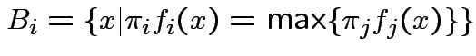
General case of ![]() populations:
populations:

Now: how would a Bayesian classify ![]() ?
?
Answer: depends on consequences and costs.
Let  be cost of classifying observation actually
from population
be cost of classifying observation actually
from population ![]() as being from population
as being from population ![]() .
.
Possible procedure: corresponds to partion of sample space into
events
 . If
. If
 classify into population
![]() .
.
Find rule to minimize expected cost; minimize

Simplest case: ![]() . Take
. Take
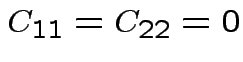 ; no cost if
you get it right.
; no cost if
you get it right.
Must minimize

Write as integral:
![\begin{multline*}
\int\left[ \pi_1 C_{12}
f_1(x)
1_{B_2}(x) \right.
\\ + \left.\pi_2 C_{21} f_2(x) \left\{1-1_{B_2}(x)\right\}\right] dx
\end{multline*}](img27.gif)
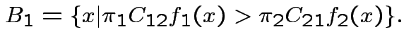
Notice that we have two choices for each ![]() : either
put
: either
put ![]() into
into  and get
 or
put it in
or
put it in  and get
 . To
minimize the integral put
. To
minimize the integral put ![]() in the one which has
the smaller corresponding value.
in the one which has
the smaller corresponding value.
That is:
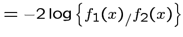
For all errors equally bad:

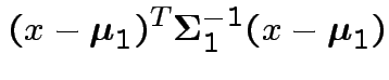
Example: Two normal populations:

Likelihood ratio is function of

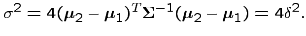
Jargon: Mahalanobis distance is

 then
is an interval and is rest.
then
is an interval and is rest.

Two dimensions some examples:
1) Both mean vectors 0.
 .
.
 diagonal with entries 2 and 1/2.
Boundaries are now
2) Same variances as in previous but now

Get


Usual rule: ![]() taken all equal and all costs
taken all equal and all costs  for
for
 . So:
. So:

Case of ![]() :
:
Notation:
 |
||
 |
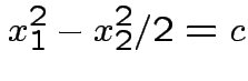
Difference in Mahalanobis distances becomes

 .
.
Rewrite as


Shape depends on eigenvalues of ![]() :
:
Both positive: ellipse
Both negative: ellipse
Opposite signs: hyperbola
 the quadratic terms cancel and
we get
the quadratic terms cancel and
we get

 and is a hyperplane.
Misclassification rates:
let ![]() denote probability under
denote probability under ![]() .
.
 assign X to $j$
 .
.


 |
||
 |

With data:
Framework: given training samples
 for
.
for
.
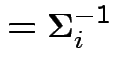
Replace
![]() in all formulas by
in all formulas by ![]() .
.
Replace
![]() in all formulas by
in all formulas by
![]() .
.
If you conclude
![]() all equal:
all equal:
Estimate using

Use Linear Discrimant analysis. Assign new ![]() to
group
to
group ![]() which minimizes
which minimizes

For ![]() rule is equivalent to assign to group 1 if
rule is equivalent to assign to group 1 if

Notice linear boundaries
Use Fisher's iris data.
Do quadratic discriminant analysis.
Use first two variables in iris data to do contouring.
Quadratic discriminant rule assigns ![]() to that group
to that group ![]() for which
for which

 pairs over the region where I wanted
to do the plotting:
pairs over the region where I wanted
to do the plotting:
nd <- 500
xvals <- seq(2.8,8,length=nd)
yvals <- seq(1.8,4.5,length=nd)
xv <- rep(xvals,nd)
yv <- rep(yvals,rep(nd,nd))
e1 <- var(diris[1:50,1:2])
e2 <- var(diris[51:100,1:2])
e3 <- var(diris[101:150,1:2])
c1 <- apply(diris[1:50,1:2],2,mean)
c2 <- apply(diris[51:100,1:2],2,mean)
c3 <- apply(diris[101:150,1:2],2,mean)
ld1<- log(prod(eigen(e1,
              symmetric=T)$values))
ld2<- log(prod(eigen(e2,
              symmetric=T)$values))
ld3<- log(prod(eigen(e3,
              symmetric=T)$values))
d1<-mahalanobis(cbind(xv,yv),c1,e1) +ld1
d2<- mahalanobis(cbind(xv,yv),c2,e2)+ld2
d3<- mahalanobis(cbind(xv,yv),c3,e3)+ld3
 is the group to which
 would be classified:
z<-rep(1,length(xv))
z[d2<d1] <- 2
z[d3<pmin(d1,d2)] <- 3
z <- matrix(z,nd,nd)
contour(xvals,yvals,z,
   levels=c(1.5,2.5),labex=0)
points(diris[1:50,1:2],pch=1)
points(diris[51:100,1:2],pch=2)
points(diris[101:150,1:2],pch=3)
Several ways if an estimated discriminant rule used.
Apparent Error Rate: Use the fitted rule to classify each observation in the training data set. Estimate
Classify as $j$Severe underestimation likely.
Parametric Estimate of Error Rate: Compute the theoretical error rates of the known parameter classifiers; plug in estimates.
Underestimation likely.
Cross validation: Delete 1 observation from the data set.
Estimate the parameters in the discriminant rule using all other
data points. Classify the deleted observation. Use fraction of
observations from population ![]() classified as
classified as ![]() to estimate
error rates.
to estimate
error rates.
Six types of glass: Window Float, Window Non-float, Vehicle, Container Tableware, Vehicle Head Lamp
Eight Response variables: all percentages by weight of oxides of: Sodium, Magnesium, Aluminum, Silicon, Potassium, Calcium, Barium and Iron.
Use Splus to do linear discriminant analysis:
glass <- read.table("fglass.dat",
             header = T)
glass$type <- as.factor(glass$type)
Notice creation of class variable.
fit <- lm(as.matrix(glass[, 1:9]) ~ type)
r <- residuals(fit)
V <- 213*var(r)/208
FV <- fitted(fit)
Means <- FV[c(1, 71, 147, 164, 177, 186),  ]
for(i in 1:214) {
 for(j in 1:6)
  Distances[i,j]<-
     mahalanobis(glass[i,1:9],
        Means[j,  ], V)
}
Notice Splus version of glm.
> summary(fit)
Response: RI
           Df Sum ofSq   Mean Sq     F    Pr(F)
     type   5 0.000073 1.46295e-05 1.609 0.1590
Residuals 208 0.001891 9.09257e-06

Response: Na
           Df Sum of Sq  Mean Sq  F Value Pr(F)
     type   5  57.80464 11.56093 28.54802     0
Residuals 208  84.23257  0.40496

Response: Mg
           Df Sum of Sq  Mean Sq  F Value Pr(F)
     type   5  271.0954 54.21908 65.54452     0
Residuals 208  172.0597  0.82721

Response: Al
           Df Sum of Sq  Mean Sq  F Value Pr(F)
     type   5  24.53088 4.906177 35.72668     0
Residuals 208  28.56366 0.137325

Response: Si
           Df SumofSq MeanSq   F    Pr(F)
     type   5   8.024 1.6048 2.787 0.0185
Residuals 208 119.759 0.5758

Response: K
           Df SumofSq MeanSq   F    Pr(F)
     type   5  15.742 3.1484 8.748 1.507e-07
Residuals 208  74.858 0.3599
Response: Ca
           Df SumofSq MeanSq  F    Pr(F)
     type   5   28.76 5.7520 2.97 0.0130
Residuals 208  402.64 1.9358

Response: Ba
           Df Sum of Sq  Mean Sq F Value Pr(F)
     type   5  25.47176 5.094353 38.9746     0
Residuals 208  27.18759 0.130710

Response: Fe
           Df SumofSq  Mean Sq  F    Pr(F)
     type   5  0.1237 0.024744 2.71 0.0214
Residuals 208  1.8986 0.009128
Variable RI (Refractive Index) could well be dropped.
Now classify training data
 Classes <- rep(1,214)
 for(i in 1:214){
  jmin <- 1
  for(j in 2:6){
   if(Distances[i,j]
       < Distances[i,jmin])
         jmin <- j
 }
 Classes[i]<- jmin
 Classmat <- matrix(0,7,7)
 for( i in 1:214){
  Classmat[glass$type[i],Classes[i]] <-
  Classmat[glass$type[i],Classes[i]]+1}
 Classmat
     [,1] [,2] [,3] [,4] [,5] [,6] [,7]
[1,]   46   14   10    0    0    0    0
[2,]   16   41   12    4    3    0    0
[3,]    3    3   11    0    0    0    0
[4,]    0    0    0    0    0    0    0
[5,]    0    2    0   10    0    1    0
[6,]    1    1    0    0    7    0    0
[7,]    0    1    1    2    1   24    0
 Classmat <- Classmat[-4,-7]
 Classmat
     [,1] [,2] [,3] [,4] [,5] [,6]
[1,]   46   14   10    0    0    0
[2,]   16   41   12    4    3    0
[3,]    3    3   11    0    0    0
[4,]    0    2    0   10    0    1
[5,]    1    1    0    0    7    0
[6,]    0    1    1    2    1   24
The error rates for linear discriminant
analysis are quite high.
Next do crossvalidation
CVClass <- rep(0,214)
for( i in 1:214){
 d <- as.matrix(glass[-i,1:9])
 tp <- as.numeric(glass[-i,10])
 mn <- matrix(0,7,9)
 for( j in c(1,2,3,5,6,7)){
 mn[j,] <- apply(d[tp==j,],2,mean)}
 mn <- mn[-4,]
 V <- var(residuals(lm(d~as.factor(tp))))
 V <- solve(V)
 dmin <- mahalanobis(glass[i,1:9],
              mn[1,],V,inverted=T)
 jmin <- 1
 for(j in 2:6)  {
  ds <- mahalanobis(glass[i,1:9],
           mn[j,],V,inverted=T)
  if( ds < dmin) { jmin<- j
      dmin <- ds
  }
 }
 CVClass[i] <- jmin
}
CVmat
      [,1] [,2] [,3] [,4] [,5] [,6]
[1,]   45   14   11    0    0    0
[2,]   17   37   12    6    3    1
[3,]    5    3    9    0    0    0
[4,]    0    0    0    0    0    0
[5,]    0    5    1    6    0    1
[6,]    1    1    0    0    6    1
[7,]    0    1    1    2    1   24
> CVmat <- CVmat[-4,]
> CVmat-Classmat
     [,1] [,2] [,3] [,4] [,5] [,6]
[1,]   -1    0    1    0    0    0
[2,]    1   -4    0    2    0    1
[3,]    2    0   -2    0    0    0
[4,]    0    3    1   -4    0    0
[5,]    0    0    0    0   -1    1
[6,]    0    0    0    0    0    0
Notice increased error rate using CV Other methods:
Classification and Regression Trees
Neural Networks
Logistic Regression
Use S function tree to classify the iris data.
First made variables from built-in data iris.
Here is my S code:
postscript("iristree.ps",horizontal=F)
variety <- as.category(c(rep("Setosa", 50),
 rep("Versicolor",50),rep("Virginica",50)))
iris.tree <- tree(variety ~ sepal.length +
 sepal.width + petal.length + petal.width)
plot(iris.tree)
text(iris.tree)
summary(iris.tree)
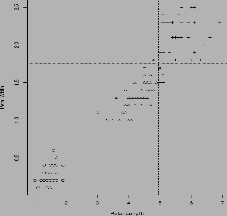
plot(petal.length,petal.width,
     xlab="Petal Length",
     ylab="Petal Width",type='n')
points(petal.length[1:50],
     petal.width[1:50], pch=1)
points(petal.length[51:100],
     petal.width[51:100], pch=2)
points(petal.length[101:150],
     petal.width[101:150], pch=3)
abline(v=2.45)
abline(h=1.75,lty=2)
abline(v=4.95,lty=3)

rt <- (petal.width < 1.75) & (variety > 1)
plot(petal.length[rt],sepal.length[rt],
  xlab="Petal Length",ylab="Sepal Length",
     type='n')
points(petal.length[rt & variety ==2],
     sepal.length[rt & variety ==2],pch=2)
points(petal.length[rt & variety ==3],
     sepal.length[rt & variety ==3],pch=3)
abline(v=4.95)
abline(h=5.15,lty=2)
dev.off()
I create the categorical variable variety to hold the labels for the three types of Iris and then essentially regress this categorical variable on the covariates shown. The function summary produces:
Classification tree:
tree(formula = variety ~ sepal.length
    + sepal.width + petal.length
    + petal.width)
Variables actually used
          in tree construction:
 "petal.length" "petal.width" "sepal.length"
Number of terminal nodes:  6
Residual mean deviance:
        0.1253 = 18.05 / 144
Misclassification error
        rate: 0.02667 = 4 / 150
Deviance: fitting multinomial model
to probability given flower comes from given species
given the covariates. Model has