Likelihood Methods of Inference

Given data $X$ with model $\{f_\theta(x);\theta\in\Theta\}$:

Definition: The likelihood function is map $L$: domain $\Theta$, values given by

$$L(\theta) = f_\theta(X)$$

Key Point: think about how the density depends on $\theta$ not about how it depends on $X$.

Notice: $X$, observed value of the data, has been plugged into the formula for density.

We use likelihood for most inference problems:

1. Point estimation: we must compute an estimate $\hat\theta = \hat\theta(X)$ which lies in $\Theta$. The maximum likelihood estimate (MLE) of $\theta$ is the value $\hat\theta$ which maximizes $L(\theta)$ over $\theta\in \Theta$ if such a $\hat\theta$ exists.

2. Point estimation of a function of $\theta$: we must compute an estimate $\hat\phi = \hat\phi(X)$ of $\phi=g(\theta)$. We use $\hat\phi=g(\hat\theta)$ where $\hat\theta$ is the MLE of $\theta$.

3. Interval (or set) estimation. We must compute a set $C=C(X)$ in $\Theta$ which we think will contain $\theta_0$. We will use
   $$\{\theta\in\Theta: L(\theta) > c\}$$
   for a suitable $c$.

4. Hypothesis testing: decide whether or not $\theta_0\in\Theta_0$ where $\Theta_0 \subset \Theta$. We base our decision on the likelihood ratio
   $$\frac{\sup\{L(\theta); \theta \in \Theta_0\}}{ \sup\{L(\theta); \theta \in \Theta\setminus\Theta_0\}}$$

Maximum Likelihood Estimation

To find MLE maximize $L$.

Typical function maximization problem:

Set gradient of $L$ equal to 0

Check root is maximum, not minimum or saddle point.

Often $L$ is product of $n$ terms (given $n$ independent observations).

Much easier to work with logarithm of $L$: log of product is sum and logarithm is monotone increasing.

Definition: The Log Likelihood function is

$$\ell(\theta) = \log\{L(\theta)\} \,.$$

Samples from MVN Population

Simplest problem: collect replicate measurements ${\bf X}_1,\ldots,{\bf X}_n$ from single population.

Model: $X_i$ are iid $MVN_p(\boldsymbol\mu, \boldsymbol\Sigma)$.

Parameters ($\theta$): $(\boldsymbol\mu, \boldsymbol\Sigma)$. Parameter space: $\boldsymbol\mu\in \mathbb {R}^p$ and $\boldsymbol\Sigma$ is some positive definite $p\times p$ matrix.

Log likelihood is

$$\ell(\boldsymbol\mu, \boldsymbol\Sigma) = -n p\log(\pi)/2 - n\log\det\boldsymbol\Sigma / 2$$

$$- \sum ({\bf X}_i -\boldsymbol\mu)^T\boldsymbol\Sigma^{-1}({\bf X}_i -\boldsymbol\mu)/2$$

Take derivatives.

$$\frac{\partial\ell}{\partial\boldsymbol\mu} = \boldsymbol\Sigma^{-1}\left\{\sum({\bf X}_i-\boldsymbol\mu)\right\}$$

$$= n\boldsymbol\Sigma^{-1}(\bar{{\bf X}}-\boldsymbol\mu)$$

where $\bar{{\bf X}}= \sum {\bf X}_i/n$. Second derivative wrt $\boldsymbol\mu$ is a matrix:

$$-n\boldsymbol\Sigma^{-1}$$

Fact: if second derivative matrix is negative definite at critical point then critical point is a maximum.

Fact: if second derivative matrix is negative definite everywhere then function is concave; no more than 1 critical point.

Summary: $\ell$ is maximized at

$$\hat{\boldsymbol\mu} = \bar{{\bf X}}$$

(regardless of choice of $\boldsymbol\Sigma$).

More difficult: differentiate $\ell$ wrt $\boldsymbol\Sigma$.

Somewhat simpler: set ${\bf D}=\boldsymbol\Sigma^{-1}$

First derivative wrt ${\bf D}$ is matrix with entries

$$\frac{\partial\ell}{\partial{\bf D}_{ij}}$$

Warning: method used ignores symmetry of $\boldsymbol\Sigma$.

Need: derivative of two functions:

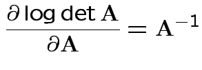
$$\frac{\partial\log\det{\bf A}}{\partial{\bf A}} = {\bf A}^{-1}$$

and

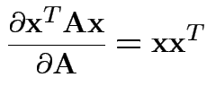
$$\frac{\partial{\bf x}^T{\bf A}{\bf x}}{\partial{\bf A}} = {\bf x}{\bf x}^T$$

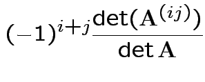
Fact: $ij^$th entry of ${\bf A}^{-1}$ is

$$(-1)^{i+j}\frac{\det({\bf A}^{(ij)})}{\det{{\bf A}}}$$

where ${\bf A}^{(ij)}$ denotes matrix obtained from ${\bf A}$ by removing column $j$ and row $i$.

Fact: $\det({\bf A})= \sum_k (-1)^{i+k} A_{ik} \det({\bf A}^{(ik)})$; expansion by minors.

Conclusion

$$\frac{\partial\log\det{\bf A}}{\partial A_{ij}} = ({\bf A}^{-1})_{ij}$$

and

$$\frac{\partial\log\det{\bf A}^{-1}}{\partial A_{ij}} = -({\bf A}^{-1})_{ij}$$

Implication

$$\frac{\partial\ell}{\partial{\bf D}} = -n\boldsymbol\Sigma/2 -\sum_i({\bf X}_i - \boldsymbol\mu)({\bf X}_i - \boldsymbol\mu)^T/2$$

Set = 0 and find only critical point is

$$\hat{\boldsymbol\Sigma} = \sum_i({\bf X}_i - \bar{{\bf X}})({\bf X}_i - \bar{{\bf X}})^T/n$$

Usual sample covariance matrix is

$${\bf S} = \sum_i({\bf X}_i - \bar{{\bf X}})({\bf X}_i - \bar{{\bf X}})^T/(n-1)$$

Properties of MLEs:

1) $\bar{{\bf X}}\sim MVN_p(\boldsymbol\mu,n^{-1}\boldsymbol\Sigma)$

2) ${\rm E}({\bf S}) = \boldsymbol\Sigma$.

Distribution of ${\bf S}$? Joint distribution of $\bar{{\bf X}}$ and ${\bf S}$?

Univariate Normal samples: Distribution Theory

Theorem: Suppose $X_1,\ldots,X_n$ are independent $N(\mu,\sigma^2)$ random variables. Then

1. $\bar X$ (sample mean)and $s^2$ (sample variance) independent.

2. $n^{1/2}(\bar{X} - \mu)/\sigma \sim N(0,1)$.

3. $(n-1)s^2/\sigma^2 \sim \chi^2_{n-1}$.

4. $n^{1/2}(\bar{X} - \mu)/s \sim t_{n-1}$.

Proof: Let $Z_i=(X_i-\mu)/\sigma$.

Then $Z_1,\ldots,Z_p$ are independent $N(0,1)$.

So $Z=(Z_1,\ldots,Z_p)^T$ is multivariate standard normal.

Note that $\bar{X} = \sigma\bar{Z}+\mu$ and $s^2 = \sum(X_i-\bar{X})^2/(n-1) = \sigma^2 \sum(Z_i-\bar{Z})^2/(n-1)$ Thus

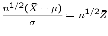
$$\frac{n^{1/2}(\bar{X}-\mu)}{\sigma} = n^{1/2}\bar{Z}$$

$$\frac{(n-1)s^2}{\sigma^2} = \sum(Z_i-\bar{Z})^2$$

and

$$T=\frac{n^{1/2}(\bar{X} - \mu)}{s} = \frac{n^{1/2} \bar{Z}}{s_Z}$$

where $(n-1)s_Z^2 = \sum(Z_i-\bar{Z})^2$.

So: reduced to $\mu=0$ and $\sigma=1$.

Step 1: Define

$$Y=(\sqrt{n}\bar{Z}, Z_1-\bar{Z},\ldots,Z_{n}-\bar{Z})^T \,.$$

(So $Y$ has dimension $n+1$.) Now

$$Y =\left[\begin{array}{cccc} \frac{1}{\sqrt{n}} & \frac{1}{\sqrt{... ...] \left[\begin{array}{c} Z_1 \\ Z_2 \\ \vdots \\ Z_n \end{array}\right]$$

or letting ${\bf M}$ denote the matrix

$$Y={\bf M}Z \,.$$

It follows that $Y\sim MVN(0,{\bf M}{\bf M}^T)$ so we need to compute ${\bf M}{\bf M}^T$:

$${\bf M}{\bf M}^T = \left[\begin{array}{c\vert cccc} 1 & 0 & 0 & \cdots & 0 \\ \hli... ...ots & -\frac{1}{n} \\ 0 & \vdots & \cdots & & 1-\frac{1}{n} \end{array} \right]$$

$$= \left[\begin{array}{c\vert c} 1 & 0 \\ \hline \\ 0 & {\bf Q} \end{array} \right] \,.$$

Put ${\bf Y}_2=(Y_2,\ldots,Y_{n+1})$. Since

$${\rm Cov}(Y_1,{\bf Y}_2) = 0$$

conclude $Y_1$ and ${\bf Y}_2$ are independent and each is normal.

Thus $\sqrt{n}\bar{Z}$ is independent of $Z_1-\bar{Z},\ldots,Z_{n}-\bar{Z}$.

Since $s_Z^2$ is a function of $Z_1-\bar{Z},\ldots,Z_{n}-\bar{Z}$ we see that $\sqrt{n}\bar{Z}$ and $s_Z^2$ are independent.

Also, see $\sqrt{n}\bar{Z}\sim N(0,1)$.

First 2 parts done.

Consider $(n-1)s^2/\sigma^2 = {\bf Y}_2^T{\bf Y}_2$. Note that ${\bf Y}_2 \sim MVN(0,{\bf Q})$.

Now: distribution of quadratic forms:

Suppose $Z\sim MVN(0,{\bf I})$ and ${\bf A}$ is symmetric. Put ${\bf A}= {\bf P}{\bf D}{\bf P}^T$ for ${\bf D}$ diagonal, ${\bf P}$ orthogonal.

Then

$${\bf Z}^T{\bf A}{\bf Z}= ({\bf Z}^*)^T {\bf D}{\bf Z}^*$$

where

$${\bf Z}^* = {\bf P}^T{\bf Z}$$

But ${\bf Z}^*\sim MVN(0,{\bf P}^T{\bf P}={\bf I})$ is standard multivariate normal.

So: ${\bf Z}^T{\bf A}{\bf Z}$ has same distribution as

$$\sum_i \lambda_i Z_i^2$$

where $\lambda_1,\ldots,\lambda_n$ are eigenvalues of ${\bf A}$.

Special case: if all $\lambda_i$ are either 0 or 1 then ${\bf Z}^T{\bf A}{\bf Z}$ has a chi-squared distribution with df = number of $\lambda_i$ equal to 1.

When are eigenvalues all 1 or 0?

Answer: if and only if ${\bf A}$ is idempotent.

1) If ${\bf A}$ idempotent and $\lambda, x$ is an eigenpair the

$${\bf A}x = \lambda x$$

and

$${\bf A}x = {\bf A}{\bf A}x = \lambda {\bf A}x = \lambda^2 x$$

so

$$(\lambda-\lambda^2) x =0$$

proving $\lambda$ is 0 or 1.

2) Conversely if all eigenvalues of ${\bf A}$ are 0 or 1 then ${\bf D}$ has 1s and 0s on diagonal so

$${\bf D}^2 = {\bf D}$$

and

$${\bf A}{\bf A}= {\bf P}{\bf D}{\bf P}^T {\bf P}{\bf D}{\bf P}^T = {\bf P}{\bf D}^2 {\bf P}^t = {\bf P}{\bf D}{\bf P}= {\bf A}$$

Next case: ${\bf X}\sim MVN_p(0,\boldsymbol\Sigma)$. Then ${\bf X}={\bf A}{\bf Z}$ with ${\bf A}{\bf A}^T=\boldsymbol\Sigma$.

Since ${\bf X}^T{\bf X}= {\bf Z}^T {\bf A}^T{\bf A}{\bf Z}$ it has the law

$$\sum \lambda_i Z_i^2$$

$\lambda_i$ are eigenvalues of ${\bf A}^T{\bf A}$. But

$${\bf A}^T{\bf A}x = \lambda x$$

implies

$${\bf A}{\bf A}^T{\bf A}x= \boldsymbol\Sigma {\bf A}x = \lambda{\bf A}x$$

So eigenvalues are those of $\boldsymbol\Sigma$ and ${\bf X}^T{\bf X}$ is $\chi^2_\nu$ iff $\boldsymbol\Sigma$ is idempotent and ${\rm trace}(\boldsymbol\Sigma)=\nu$.

Our case: ${\bf A}={\bf Q}= {\bf I}- {\bf 1}{\bf 1}^T/n$. Check ${\bf Q}^2 = {\bf Q}$. How many degrees of freedom: ${\rm trace}({\bf D})$.

Defn: The trace of a square matrix ${\bf A}$ is

$${\rm trace}({\bf A}) = \sum {\bf A}_{ii}$$

Property: ${\rm trace}({\bf A}{\bf B})={\rm trace}({\bf B}{\bf A})$.

So:

$${\rm trace}({\bf A}) ={\rm trace}({\bf P}{\bf D}{\bf P}^T)$$

$$={\rm trace}({\bf D}{\bf P}^T{\bf P}) = {\rm trace}({\bf D})$$

Conclusion: df for $(n-1)s^2/\sigma^2$ is

$${\rm trace}( {\bf I}- {\bf 1}{\bf 1}^T/n) = n-1.$$

Derivation of the $\chi^2$ density:

Suppose $Z_1,\ldots,Z_n$ independent $N(0,1)$. Define $\chi^2_n$ distribution to be that of $U=Z_1^2 + \cdots + Z_n^2$. Define angles $\theta_1,\ldots,\theta_{n-1}$ by

$$Z_1 = U^{1/2} \cos\theta_1$$

$$Z_2 = U^{1/2} \sin\theta_1\cos\theta_2$$

$$\vdots = \vdots$$

$$Z_{n-1} = U^{1/2} \sin\theta_1\cdots \sin\theta_{n-2}\cos\theta_{n-1}$$

$$Z_n = U^{1/2} \sin\theta_1\cdots \sin\theta_{n-1} \,.$$

(Spherical co-ordinates in $n$ dimensions. The $\theta$ values run from 0 to $\pi$ except last $\theta$ from 0 to $2\pi$.) Derivative formulas:

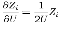
$$\frac{\partial Z_i}{\partial U} = \frac{1}{2U} Z_i$$

and

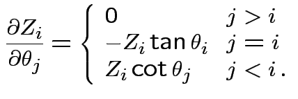
$$\frac{\partial Z_i}{\partial\theta_j} = \left\{ \begin{array}{ll}... ...\ -Z_i\tan\theta_i & j=i \\ Z_i\cot\theta_j & j < i \,. \end{array}\right.$$

Fix $n=3$ to clarify the formulas. Use shorthand $R=\sqrt{U}$.

Matrix of partial derivatives is

$$\left[\begin{array}{ccc} \frac{\cos\theta_1}{2R} & -R \sin\theta_... ...R \cos\theta_1\sin\theta_2 & R \sin\theta_1\cos\theta_2 \end{array}\right] \,.$$

Find determinant:

$$U^{1/2}\sin(\theta_1)/2$$

(non-negative for all $U$ and $\theta_1$). General $n$: every term in the first column contains a factor $U^{-1/2}/2$ while every other entry has a factor $U^{1/2}$.

FACT: multiplying a column in a matrix by $c$ multiplies the determinant by $c$.

SO: Jacobian of transformation is

$$u^{(n-2)/2}u^{-1/2}/2 \times h(\theta_1,\theta_{n-1})$$

for some function, $h$, which depends only on the angles.

Thus joint density of $U,\theta_1,\ldots \theta_{n-1}$ is

$$(2\pi)^{-n/2} \exp(-u/2) u^{(n-2)/2}h(\theta_1, \cdots, \theta_{n-1}) / 2 \,.$$

To compute the density of $U$ we must do an $n-1$ dimensional multiple integral $d\theta_{n-1}\cdots d\theta_1$.

Answer has the form

$$cu^{(n-2)/2} \exp(-u/2)$$

for some $c$.

Evaluate $c$ by making

$$\int f_U(u) du = c \int_0^\infty u^{(n-2)/2} \exp(-u/2) du$$

$$=1.$$

Substitute $y=u/2$, $du=2dy$ to see that

$$c 2^{n/2} \int_0^\infty y^{(n-2)/2}e^{-y} dy = c 2^{n/2} \Gamma(n/2)$$

$$=1.$$

CONCLUSION: the $\chi^2_n$ density is

$$\frac{1}{2\Gamma(n/2)} \left(\frac{u}{2}\right)^{(n-2)/2} e^{-u/2} 1(u>0) \,.$$

Fourth part: consequence of first 3 parts and def'n of $t_\nu$ distribution.

Defn: $T\sim t_\nu$ if $T$ has same distribution as

$$Z/\sqrt{U/\nu}$$

for $Z\sim N(0,1)$, $U\sim\chi^2_\nu$ and $Z,U$ independent.

Derive density of $T$ in this definition:

$$P(T \le t) = P( Z \le t\sqrt{U/\nu})$$

$$= \int_0^\infty \int_{-\infty}^{t\sqrt{u/\nu}} f_Z(z)f_U(u) dz du$$

Differentiate wrt $t$ by differentiating inner integral:

$$\frac{\partial}{\partial t}\int_{at}^{bt} f(x)dx = bf(bt)-af(at)$$

by fundamental thm of calculus. Hence

$$\frac{d}{dt} P(T \le t) = \int_0^\infty \frac{f_U(u)}{ \sqrt{2\pi}} \left(\frac{u}{\nu}\right)^{1/2} \exp\left(-\frac{t^2u}{2\nu}\right) du \,.$$

Plug in

$$f_U(u)= \frac{1}{2\Gamma(\nu/2)}(u/2)^{(\nu-2)/2} e^{-u/2}$$

to get

$$f_T(t) = \frac{\int_0^\infty (u/2)^{(\nu-1)/2} e^{-u(1+t^2/\nu)/2} du }{2\sqrt{\pi\nu}\Gamma(\nu/2)} \,.$$

Substitute $y=u(1+t^2/\nu)/2$, to get

$$dy=(1+t^2/\nu)du/2$$

$$(u/2)^{(\nu-1)/2}= [y/(1+t^2/\nu)]^{(\nu-1)/2}$$

leading to

$$f_T(t) = \frac{(1+t^2/\nu)^{-(\nu+1)/2} }{\sqrt{\pi\nu}\Gamma(\nu/2)} \int_0^\infty y^{(\nu-1)/2} e^{-y} dy$$

or

$$f_T(t)= \frac{\Gamma((\nu+1)/2)}{\sqrt{\pi\nu}\Gamma(\nu/2)}\frac{1}{(1+t^2/\nu)^{(\nu+1)/2}} \,.$$

Multivariate Normal samples: Distribution Theory

Theorem: Suppose ${\bf X}_1,\ldots,{\bf X}_n$ are independent $N(\boldsymbol\mu,\boldsymbol\Sigma)$ random variables. Then

1. $\bar {\bf X}$ (sample mean)and ${\bf S}$ (sample variance-covariance matrix) are independent.

2. $n^{1/2}(\bar{{\bf X}} - \boldsymbol\mu)\sim MVN(0,{\bf I})$.

3. $(n-1){\bf S}\sim {\rm Wishart}_p(n-1,\boldsymbol\Sigma)$.

4. $T^2=n(\bar{{\bf X}} - \boldsymbol\mu)^T{\bf S}^{-1}(\bar{{\bf X}} - \boldsymbol\mu)$ is Hotelling's $T^2$. $(n-p)T^2/(p(n-1))$ has an $F_{p,n-p}$ distribution.

Proof: Let ${\bf X}_i={\bf A}{\bf Z}_i+\boldsymbol\mu$ where ${\bf A}{\bf A}^T=\boldsymbol\Sigma$ and ${\bf Z}_1,\ldots,{\bf Z}_p$ are independent $MVN(0,{\bf I})$.

So ${\bf Z}=({\bf Z}_1^T,\ldots,{\bf Z}_p^T)^T \sim MVN_p(0,{\bf I})$.

Note that $\bar{{\bf X}} = {\bf A}\bar{{\bf Z}}+\boldsymbol\mu$ and

$$(n-1){\bf S} = \sum({\bf X}_i-\bar{{\bf X}})({\bf X}_i-\bar{{\bf X}})^T$$

$$= {\bf A}\sum({\bf Z}_i-\bar{{\bf Z}})({\bf Z}_i-\bar{{\bf Z}})^T{\bf A}^T$$

Thus

$$n^{1/2}(\bar{X}-\mu) = {\bf A}n^{1/2}\bar{{\bf Z}}$$

and

$$T^2 =\left(n^{1/2}\bar{{\bf Z}}\right)^T {\bf S}_{\bf Z}^{-1}\left(n^{1/2}\bar{{\bf Z}}\right)$$

where

$${\bf S}_Z= \sum({\bf Z}_i-\bar{{\bf Z}})({\bf Z}_i-\bar{{\bf Z}})^T/(n-1).$$

Consequences. In 1, 2 and 4: can assume $\boldsymbol\mu=0$ and $\boldsymbol\Sigma={\bf I}$. In 3 can take $\boldsymbol\mu=0$. Step 1: Do general $\boldsymbol\Sigma$. Define

$${\bf Y}=(\sqrt{n}\bar{{\bf Z}}^T, {\bf Z}_1^T-\bar{{\bf Z}}^T,\ldots, {\bf Z}_{n}^T-\bar{{\bf Z}}^T)^T \,.$$

(So ${\bf Y}$ has dimension $p( n+1)$.) Clearly ${\bf Y}$ is $MVN$ with mean 0.

Compute variance covariance matrix

$$\left[\begin{array}{cc} {\bf I}_{p\times p} & 0 \\ 0 & {\bf Q}^* \end{array}\right]$$

where ${\bf Q}^*$ has a pattern. It is a $p\times p$ patterned matrix with entry $ij$ being

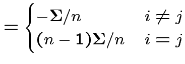
$${\rm Cov}({\bf Z}_i- \bar{{\bf Z}},{\bf Z}_j- \bar{{\bf Z}}) = \begin{cases}-\boldsymbol\Sigma/n & i \neq j \\ (n-1)\boldsymbol\Sigma/n & i=j \end{cases}$$

$$= {\bf Q}_{ij}\boldsymbol\Sigma$$

Kronecker Products

Defn: If ${\bf A}$ is $p \times q$ and ${\bf B}$ is $r \times s$ then ${\bf A}\bigotimes{\bf B}$ is the $pr \times qs$ matrix with the pattern

$$\left[\begin{array}{cccc} {\bf A}_{11}{\bf B}& {\bf A}_{12}{\bf B... ...{\bf B}& {\bf A}_{p2} {\bf B}& \cdots & {\bf A}_{pq}{\bf B} \end{array}\right]$$

So our variance covariance matrix is

$${\bf Q}^* = {\bf Q}\bigotimes \boldsymbol\Sigma$$

Conclusions so far:

1) $\bar{{\bf X}}$ and ${\bf S}$ are independent.

2) $\sqrt{n}(\bar{{\bf X}} - \boldsymbol\mu ) \sim MVN(0,\boldsymbol\Sigma)$

Next: Wishart law.

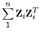
Defn: The ${\rm Wishart}_p(n,\boldsymbol\Sigma)$ distribution is the distribution of

$$\sum_1^n {\bf Z}_i{\bf Z}_i^T$$

where ${\bf Z}_1,\ldots,{\bf Z}_n$ are iid $MVN_p(0,\boldsymbol\Sigma)$.

Properties of Wishart.

1) If ${\bf A}{\bf A}^t=\boldsymbol\Sigma$ then

$${\rm Wishart}_p(0,\boldsymbol\Sigma) = {\bf A}{\rm Wishart}_p(0,{\bf I}){\bf A}^T$$

2) if ${\bf W}_i, i=1,2$ independent ${\rm Wishart}_p(n_i,\boldsymbol\Sigma)$ then

$${\bf W}_1+{\bf W}_2 \sim {\rm Wishart}_p(n_1+n_2,\boldsymbol\Sigma).$$

Proof of part 3: rewrite

$$\sum ({\bf Z}_i-\bar{{\bf Z}})({\bf Z}_i-\bar{{\bf Z}})^T$$

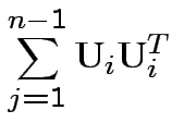
in form

$$\sum_{j=1}^{n-1} {\bf U}_i{\bf U}_i^T$$

for ${\bf U}_i$ iid $MVN_p(0,\boldsymbol\Sigma)$. Put ${\bf Z}_1,\ldots,{\bf Z}_n$ as cols in matrix ${\bf Z}$ which is $p\times n$. Then check that

$${\bf Z}{\bf Q}{\bf Z}^T = \sum ({\bf Z}_i-\bar{{\bf Z}})({\bf Z}_i-\bar{{\bf Z}})^T$$

Write ${\bf Q}= \sum {\bf v}_i {\bf v}_i^T$ for $n-1$ orthogonal unit vectors ${\bf v}_1,\ldots,{\bf v}_{n-1}$. Define

$${\bf U}_i = {\bf Z}{\bf v}_i$$

and compute covariances to check that the ${\bf U}_i$ are iid $MVN_p(0,\boldsymbol\Sigma)$. Then check that

$${\bf Z}{\bf Q}{\bf Z}^T = \sum{\bf U}_i{\bf U}_i^T$$

Proof of 4: suffices to have $\boldsymbol\Sigma={\bf I}$.

Uses further props of Wishart distribution.

3: If ${\bf W}\sim Wishart_p(n,\boldsymbol\Sigma)$ and ${\bf a}\in \mathbb {R}$ then

$$\frac{{\bf a}^T {\bf W}{\bf a}}{{\bf a}^T\boldsymbol\Sigma {\bf a}} \sim \chi_n^2$$

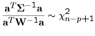
4: If ${\bf W}\sim Wishart_p(n,\boldsymbol\Sigma)$ and $n \ge p$ then

$$\frac{ {\bf a}^T\boldsymbol\Sigma^{-1} {\bf a} }{ {\bf a}^T {\bf W}^{-1} {\bf a} } \sim \chi_{n-p+1}^2$$

5: If ${\bf W}\sim Wishart_p(n,\boldsymbol\Sigma)$ then

$${\rm trace}(\boldsymbol\Sigma^{-1}{\bf W}) \sim \chi_{np}^2$$

6: If ${\bf W}\sim Wishart_{p+q}(n,\boldsymbol\Sigma)$ is partitioned into components then

$${\bf W}_{11} - {\bf W}_{12}{\bf W}_{22}^{-1} {\bf W}_{21} \sim Wishart_{p}(n-q,\boldsymbol\Sigma_{11.2})$$