STAT 804: Lecture 1 Examples

Some time series

Comments on the data sets:

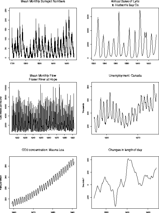
• Top left: Sunspot data. Each month the average number of sunspots is recorded. Notice the apparent periodicity, the large variability when the series is at a high level and the small variability when the series is at a small level. This series is likely to be quite stationary over the time span we have been able to observe it, though it may have a nearly perfectly periodic component.

• Top right: Annual sales of lynx pelts to the Hudson's Bay Company. There is a clear cycle of about 10 years in length. Might there be a longer term cycle? Is the cycle produced by a strictly periodic phenomenon or by a dynamic system close to a periodic system?

• Middle left: Mean monthly flow rates for the Fraser River at Hope. There are signs of lower variability at low levels suggesting transformation. There is a clear annual cycle which will have to be removed to look for stationary residuals.

• Middle right: Monthly unemployment numbers in Canada. Notice the probably presence of a slow upward trend; such a trend should be present in the presence of a growing population. This series is not stationary. The trend is not too linear with some apparent long term cycles perhaps which produce an S shaped curve.

• Lower left: Carbon Dioxide above Mauna Loa (a Hawaian volcano). There is a clear trend and an annual cycle but you might well hope that after compensating for these the remainder would be stationary.

• Lower right: Changes in the length of the Earth's day. This sort of very smooth graph with long runs going up and down suggests integration. We will look at differencing as a method of producing a series with less long range dependence.

I made these plots with S-Plus using the following code:

postscript("tsplots.ps",horizontal=F)
par(mfrow=c(3,2))
tsplot(sunspots,main="Mean Monthly Sunspot Numbers")
tsplot(lynx, main="Annual Sales of Lynx\n to Hudson's Bay Co.")
tsplot(flow, ylab="Cubic Meters per Second",main="Mean Monthly Flow\nFraser River at Hope")
tsplot(unemployment, main="Unemployment: Canada",ylab="Thousands")
tsplot(co2, main="CO2 concentration: Mauna Loa",ylab="Parts per Million")
tsplot(changes, main="Changes in length of day", ylab="Seconds?")
dev.off()