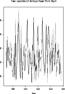
Built into S-Plus are two time series rain.nyc1 and rain.nyc2. These series are each supposed to be annual rain falls in New York in inches. Here is a plot of the series:

I used S to do plotting, model identification and fitting
#
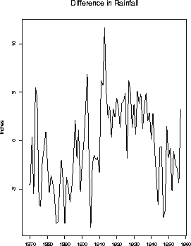
# Time series x is the difference between two rain fall series
#  for New York
#
postscript("raindiff.ps",horizontal=F)
tsplot(x,ylab="Inches",main="Difference in Rainfall")
dev.off()
This produces the following plot:

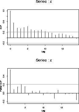
Now I plot the ACF and PACF:
postscript("raindiff_acf.ps",horizontal=F)
par(mfrow=c(2,1))
acf(x)
acf(x,type="partial")
dev.off()
which gives me:

The PACF is more or less negligible after lag 1 and so I begin with an AR(1) fit
> x.arywft <- ar(x,order.max=1)
> x.arywft$ar         # estimated ar coefficient

, , 1
         [,1]
[1,] 0.552542
> x.arywft$var.pred   # estimated noise (or prediction) variance
         [,1]
[1,] 13.45628
The same model can be fitted using the general ARIMA fitting function
arima.mle:
#
#   You must remove a mean from x or put in a regression
#    term explicitly.  The model is specified by a list
#     Here I specify an ARIMA(1,0,0) model. Much more
#     general models are possible.
#
> x.armlft <- arima.mle(x-mean(x),model=list(order=c(1,0,0)))
#
#  The result is a list with many components including
#
> x.armlft$model
$order:
[1] 1 0 0

$ar:
[1] 0.5572896

$ndiff:
[1] 0
#
#  You see that the autoregression coefficient is slightly different
#   as is the estimated error variance
#
> x.armlft$sigma2
[1] 13.0793
#
#  Finally the estimated variance of the fitted coefficient is
#
> x.armlft$var.coef
            ar(1)
ar(1) 0.007834412
You get the same result from the code
> arima.mle(x,xreg=rep(1,length(x)),model=list(order=c(1,0,0)))some of whose output is
$model$ar:
[1] 0.5574448

$var.coef:
            ar(1)
ar(1) 0.007832446

$sigma2:
[1] 13.07461
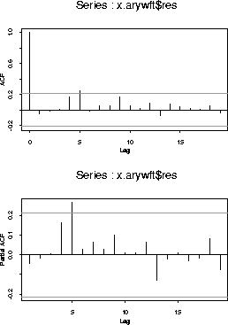
Next I plotted the autocorrelation function of the residuals which are part of the fit.
postscript("raindiff_resid_acf.ps",horizontal=F)
par(mfrow=c(2,1))
acf(x.arywft$res)
acf(x.arywft$res,type="partial")
dev.off()
giving the plot:

The plots suggest some problem at lag 5. This coefficient is not very significant however, and hard to attach any physical meaning to so I prefer to regard it as sampling variation.