School of Communication,
Simon Fraser University,
Burnaby, BC Canada
We consider several network analysis programs/procedures that do (or could)make use of eigendecomposition methods. These will include Correspondence Analysis (CA), NEGOPY, CONCOR, CONVAR, Bonacich centrality, and certain approaches to structural equivalence. We describe the procedures these analytic approaches use and consider these procedures from a variety of perspectives. We consider the results produced by the various approaches and examine the similarities and differences between them in terms of what they tell the user about networks and what it is about the procedures that is the source of the strengths and weaknesses of the methods.
Network analysis begins with data that describes the set of relationships among the members of a system. The goal of analysis is to obtain from the low-level relational data a higher-level description of the structure of the system. The higher-level description identifies various kinds of patterns in the set of relationships. These patterns will be based on the way individuals are related to other individuals in the network. Some approaches to network analysis look for clusters of individuals who are tightly connected to one another; some look for sets of individuals who have similar patterns of relations to the rest of the network.
Other methods don't "look for" anything in particular -- instead, they construct a continuous multidimensional representation of the network in which the coordinates of the individuals can be further analyzed to obtain a variety of kinds of information about them and their relation to the rest of the network. One approach to this is to choose a set of axes in the multidimensional space occupied by the data and rotate them so that the first axis points in the direction of the greatest variability in the data; the second one, perpendicular to the first, points in the direction of greatest remaining variability, and so on. This set of axes is a coordinate system that can be used to describe the relative positions of the set of points in the data. Most of the variability in the locations of points will be accounted for by the first few dimensions of this coordinate system. The coordinates of the points along each axis will be an eigenvector, and the length of the projection will be an eigenvalue.
Researchers who use methods like Correspondence Analysis or principle components analysis are generally aware that they are using eigen decomposition methods. Those who use computer programs such as CONCOR or NEGOPY, however, may not be aware of this because the eigenvalues or eigenvectors are hidden more or less deeply within the analytic package. Nevertheless, eigen methods lie at the heart of these analytic tools.
Network researchers have used eigen decomposition methods either implicitly or explicitly since the late 1960's, when computers became generally accessible in most universities. In the last twenty years there has been an increasing use of these methods which have become available on microcomputers.
Some methods of analysis work by means of a direct analytic procedure in which a set of equations are used to directly calculate an exact result. Others use an iterative procedure that (hopefully) converges to an acceptable solution.
Iterative methods for the extraction of eigenvectors take one of two forms, the power method and iterated calculation.
If an adjacency matrix for a connected network that is not bipartite is raised to higher and higher powers, it will eventually converge so that the columns will be multiples of one another and of the eigenvector that belongs to the largest eigenvalue, which will be positive and unique.
There are a few problems with this naive power method:
If the largest positive eigenvalue is not exactly equal to 1.0 (a very likely case), the numbers in the matrix get either larger or smaller with each multiplication as higher powers are calculated. Very large and very small numbers can be difficult to work with and are likely to reduce the level of accuracy of the results.
For these reasons this method is generally avoided.
Another approach of this form is to repeatedly perform a calculation on the adjacency matrix, or a suitably prepared version thereof, until the result stops changing. For example, the ovariance or correlation can be calculated between pairs of columns to produce a new matrix in which the i,j cell is the covariance (or correlation) of column i with column j. The resulting matrix is subjected to the same procedure, etc., until covergence is achieved.
Iterated covariance (CONVAR) produces the same result that would be obtained with the power method applied to an adjacency matrix that has had the row and column means subtracted from all its elements. (A more complete decomposition would be obtained if this prepared matrix were subjected to a standard eigendecomposition routine.) The columns of the matrix are once again multiples of the largest eigenvector of the adjacency matrix which has had the row and column means subtracted.
When covariance is replaced with correlation (CONCOR), something different happens. Because correlation requires deviation scores to be standardized by division by standard deviation, the end result is a (nearly) binary matrix that partitions the network into two subsets. It is not possible to extract eigenvectors or values with iterated corelation; CONCOR requires the full matrix as does the naive power method. Since CONCOR is a nonlinear process, the results are difficult to interpret.
An alternative method that produces results exactly equivalent those of the naive power method is to multiply a random vector by the adjacency matrix again and again rather than multiplying the matrix by itself. This procedure makes it possible to extract eigenvectors from very large matrices while being efficient in both time and space, since the full matrix does not need to be stored in memory at any time.
One or more of the following adjustments may be made after each multiplication by the matrix. Each has an impact on the final result and the kind of information about the network it contains.
Rescaling
After each iteration, the vector is rescaled to offset the expansion or shrinkage seen in the naive power method. Convergence to the eigenvector can be detected by monitoring the size of this correction: when it stops changing from iteration to iteration, it will be equal to the eigenvalue and the process will be finished. If this is the only adjustment made, the result will be the Frobenius eigenvector (used as Bonacich Centrality in UCINET).
Centering
Another change can be seen from iteration to iteration: a "drift" in the positive or negative direction. This can be cancelled by centering the vector after each iteration. This may be achieved by subtracting the mean of the vector from its elements. Because this is equivalent to converting the values in the matrix to deviation scores by removal of means, the result will be convergence to the first CONVAR eigenvector and value.
Normalizing
While multiplying the vector by the matrix, one may also divide each component of the vector by the corresponding matrix row sum. When this is done in addition to rescaling and centering, the resulting eigenvector and value will be the first non-trivial Correspondence Analysis pair.
Balancing
If, in addition to the above adjustments, each node is given weight equal to its row sum in the matrix-vector multiplication, the resulting eigenvector will be the one corresponding to the first non-trivial positive eigenvalue of Correspondence Analysis. This eigenvector is associated with on-diagonal clustering. This is the procedure used by NEGOPY (although not to convergence).
The Power Method only provides the first eigenvector and value. To obtain subsequent pairs, the previous ones must be subtracted from the matrix before each set of iterations. This procedure, called "deflation," can also be done efficiently with sparse matrix techniques. Extra storage is needed only for each eigenvector and value. Beyond the first several eigenvector-value pairs, rounding error reduces the accuracy below acceptable limits.
Centering, normalizing, and balancing can also be used with general purpose eigendecomposition routines. Centering operations destroy sparsity, but this isn't an issue with routines such as the SVD program in SPSS, which use the entire matrix anyhow. Special purpose sparse-matrix routines, such as the Lanczos algorithm, allow the user to define matrix vector multiplication such that the adjustments used in the power method can be applied.
There is a fair bit of confusion about the balancing procedures we have described above. It seems that there are two major ssues:
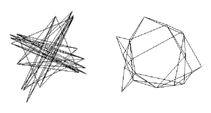
Positive eigenvalues are associated with clustering of interconnected nodes and negative ones with partitioning of the network into sets of nodes that have similar patterns of connections with nodes in other sets, but few connections amongst themselves. Because CONCOR identifies structures associated with both positive and negative eigenvalues, it is useful for identifying sets of structurally equivalent nodes -- those who have similar patterns of connections with nodes in other sets. Analysts who avoid negative eigenvalues will be unable to detect structures associated with negative eigenvalues, a form of structuring that is as important as that which is associated with positive ones. See Figure 1.
In this section we will attempt to address some practical matters. For the large sparse arrays typical of social networks, it is not likely that we will want a complete eigen decomposition, for two reasons:
The centering, balancing, and normalizing in NEGOPY are done on the fly during iterations of p' <-- Mp, where the initial p is a random vector and M is the row-normalized adjacency matrix.
Complete eigen decomposition is O(n3), and thus impractical for large networks. What would we do with all the results? A complete decomposition would give n-1 eigenvectors and an equal number of eigenvalues. This will actually be more numbers than were in the original data! We already know that a few axes will probably contain most of the important information, so why not stop after two or three dimensions? Chi-squared can be calculated once and used as a guide for how much of the structure has been explained.
We have suggested that Power Method with Deflation is a useful way to obtain the first few eigenvectors, and for large sparse arrays, and two or three dimensions, it's really not that bad. A few hundred iterations of p' <-- Mp gives the first non-trivial dimension F2 and its corresponding eigenvalue  2. A few hundred more of p' <-- Mp - 2 F2 gives the second, and that may be all that is necessary to get a reasonably informative "global" view of the structure of the network. There are more clever, faster methods of finding the first few dimensions, such as the Lanczos method.
We have used iteration of p' <-- Mp to extract the eigenvectors of a network. The fact that M is stochastic suggests that, in the long run, there will be a stable configuration. But in the short run, p will be most affected by the largest (in the senses explored in the last section) structural features. The graphs in Figure 2 show the squared correlations of p with the first four (non-trivial) eigenvectors.
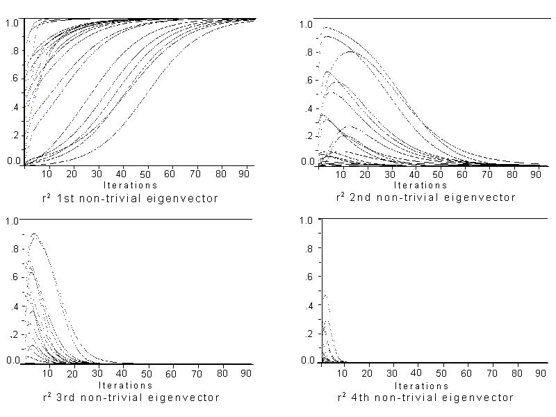
There is a fairly wide range of variation evident in these graphs. With some starting configurations convergence is rapid, requiring only five to six iterations for all but the largest eigenvector to drop out of the picture. With other configurations, a hundred or more iterations may be required. This variation is due to the fact that a random starting configuration may result in a p that points in the direction of one of the eigenvectors. If it points in the direction of the largest one, convergence will be rapid, while if it points in the direction of another, it will take more iterations. In fact, if p happens to be one of the other eigenvectors, iterating may not change the position vector at all.
To make partial iteration a useful tool, we propose choosing an initial p that is orthogonal to the largest eigenvector. Since the largest eigenvector will be the positive constant determined by the matrix of expecteds, a vector containing whole number values ranging from -n/2 to n/2 (for even n) or -(n-1)/2 to (n-1)/2 (for odd n) will be suitable. This initial p will have moderately large correlations with several eigenvectors, and will converge smoothly over a moderate number of iterations, as illustrated by Fig. 3.
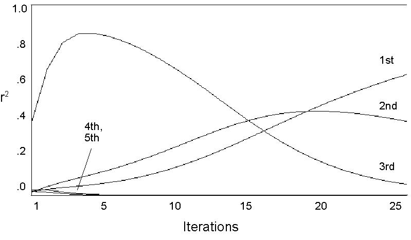
We can use this idea to devise a "divide- and-conquer" strategy for quick analysis of the main network structures. The Spectral Decomposition of M shows that after a few p' <-- Mp iterations, the vector p will consist mostly of the contributions of the most "important" eigenvectors. (Fig 3). In effect, we are projecting the ith iteration of M upon a single dimension. Now order p by the magnitudes of its components. Since each eigenvector induces a partition on p, we would expect to see the components of the ordered p changing rapidly where an important eigenvector induces a partition. We can make these partitions clearer by looking at the first difference of ordered p, as shown in Figure 4. A more sophisticated pattern-recognition approach is used in NEGOPY.
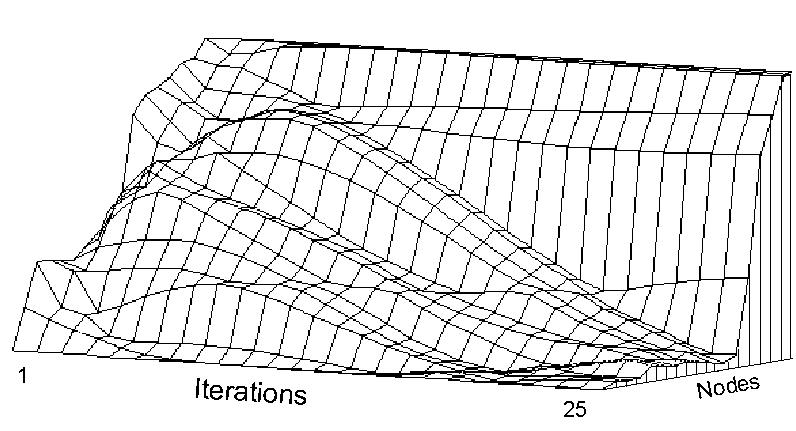
Where the first difference of ordered p is relatively constant, we would expect to find a cluster, and now we can search the sparse array for the nodes defined by this cluster, and perform any tests we wish to define "closeness", "group membership", and so on. Each induced partition is examined in turn. Of course, we must subtract off the direction associated with the "trivial" eigenvector at each step of the iteration, but this is very easy to do even with a large sparse matrix.
We presented an introductory overview of eigen analysis methods and their applications to network analysis. We showed how many popular analytic procedures (eg. CONCOR, NEGOPY, Correspondence Analysis) are at their core eigen decomposition procedures. CONVAR, because it uses covariance rather than correlation has some advantages over the closely related CONCOR. We considered alternatives to complete eigendecomposition from several perspectives: iterative approaches like the Power Method make it possible to extract eigenvectors and values from very large networks. A variety of centering, normalizing, and balancing procedures carried out prior to or during the analysis were reviewed. We showed how these procedures influence the results obtained by eigen decomposition. The effect balancing operations have on the eigenvalues was examined and the role played by negative eigenvalues and their associated vectors was briefly discussed. Finally, we examined partial decomposition strategies and showed how they make it possible to extract information about the structure of a network in an efficient and practical manner.
Barnett, G.A. (1989). Approaches to non-Euclidean network analysis. In M. Kochen (ed.). Small world. Norwood, NJ: Ablex.(pp.349-372).
Gould, P. (1967). The Geographical Interpretation of Eigenvalues" Institute of British Geographers Transactions, 42: 53-85.
Parlett, B. (1979). "The Lanczos algorithm with selective orthogonalization" Mathematics of Computation, 33:145, 217-238.
Tinkler, K. (1972). The Physical Interpretation of Eigenfunctions of Dichotomous Matrices. Inst. Br. Geog. Trans. 55,17-46.
Wasserman, S., Faust, K., and Glaskiewicz, J. (1989). Correspondence and canonical analysis of relational data.J. Mathematical Sociology. 1:1, 11-64.
Weller, S., Romney, A. (1990). Metric Scaling: Correspondence Analysis. Beverly Hills: Sage.