Use the data for the first two courses for Questions 1 - 11. Use the data for the 3rd and 4th courses for Questions 12 - 16.

1. Calculate the means and standard deviations of the scores in the first two courses.

2. Calculate Pearson's r for the scores in the first two courses.

r = .765312

3. Calculate a regression equation, using the scores on the first course as the independent variable and the scores on the second course as the dependent variable.

First the slope:

Then the intercept:

Now the equation:

4. Draw a scatterplot for the data for the first two courses and draw the regression line on the graph. Label the Y-intercept.

5. Locate the means of the first two courses on the graph and determine whether the regression line passes through the two means.

6. What is the coefficient of determination for the data for the first two courses? What does it mean?

This means that 58.57% of the variance in scores on the exam for Course 2 are accounted for or explained by the relationship with scores for Course 1. A higher correlation between the two variables would have resulted in a higher coefficient of determination. A perfect correlation (r = 1.00) would explain 100% of the variance. If the variables are not related to one another (r = 0.00), the correlation would explain none (0.0%) of the variance. Although the data points are not actually on the line, you can see that the line does seem to reasonably describe the overall relation between scores on the first and second courses. Also, if you know a student's score on the first course, you can make a reasonably accurate estimate of that student's score on the second course. Thus, you have explained some of the variation in scores on the second course by knowing the student's score on the first course.

7. What is the slope of the regression line? What does the slope tell you about your variables and how they are related to one another?

slope = .765312

This tells you that you would expect a student who gets a score 1 point higher than another on the first course to get a score .765312 points higher than the other on the second course. Since the slope is positive, higher scores on the first course are associated with higher scores on the second course.

8. Calculate the residuals for students c, f, g, and k.

In the graph above, the data points for the selected students are circled in red. The errors of prediction (residuals) are indicated by dotted blue lines.The "errors" between where the data points are and where the regression equation would predict them to be (errors of prediction) are called residuals or unexplained variation. These "errors" are what would be left over if the effect of the scores for the first course were to be "statistically removed." They are variations in the dependent variable that are not accounted for by the independent variable.

9. If the correlation between the scores in the first two courses was lower, what effect would this have on the residuals?

The scatterplots below show data where the correlations are 0.6 and 0.95. Notice that the data points in the plot with the higher correlation are much closer to the regression line. This illustrates the direct relationship between the correlation and the residuals: the closer the correlation is to 0.0, the larger the residuals will be. Alternatively, the closer the correlation is to 1.0 or -1.0, the smaller the residuals will be. This shows that stronger correlations explain more of the variability (variance) in the data.

r = 0.6 r2 = .36	r = 0.95 r2 = .9025

10. If a student received a score of 50 in the first course, what would you expect the student's score in the second course would be?

You would expect it to be:

which is:

11. If a student received a score of 100 in the first course, what would you expect the student's score in the second course would be?

12. Calculate the means and standard deviations of the scores in the third and fourth courses.

	Course 3	Course 4
a	42.66	81.68
b	85.62	49.51
c	75.3	75.39
d	43.46	77.61
e	85.74	31.82
f	41.72	84.59
g	85.53	61.88
h	85.39	63.45
i	43.25	79.94
j	85.48	70.79
k	84.02	74.35
l	41.54	96.99

	Course 3 x	Course 4 y
means	66.6425	70.6667
standard deviations (with n)	20.566785	16.492728
standard deviations (with n-1)	21.481307	17.226093

13. Calculate Pearson's r for the scores in the third and fourth courses.

r = -0.73388

14. Calculate a regression equation, using the scores on the third course as the independent variable and the scores on the fourth course as the dependent variable.

First the slope:

Then the intercept:

Now the equation:

15. Draw a scatterplot for the data for the third and fourth courses and draw the regression line on the graph. Label the Y-intercept.

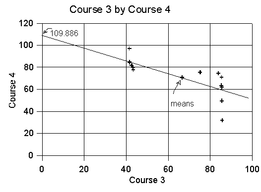
16. After looking at the scatterplot from Question 15, discuss the appropriateness of the analysis you did in Question 14. What is the problem? What are the consequences of doing this kind of analysis on data like the data for the third and fourth courses?

The relationship between the two variables in this analysis is not a linear one. A straight regression line does not fit the data well at all. Linear regression is not appropriate for this data.