Chapter 18. Tests for correlations
1. You do a survey of a sample of 82 of your fellow students and ask about how much coffee they drink and how much sleep they get on a typical night. You calculate Pearson's r for the data and find a correlation of 0.22. You would like to know if this correlation could be due to sampling variability.
a. What are your null and alternate hypotheses?


b. What test do you perform?
You perform a t-test for the significance of a correlation.
c. Assume the 95% confidence level is okay. What is the critical value? How do you determine that?
You use Table 2, Critical Values of t. Unlike z-tests, which do not consider sample size, t-tests do. In order to read Table 2, you have to compute degrees of freedom for your data. This is easy to do for t, because the degrees of freedom is your sample size minus 2: df = n - 2. For your data, where the sample size is 82, df = 80.
Because you want the 95% confidence level, you want the column in the table for the .05 level of significance. You will see that there are two columns for this level – the second and third ones. Because you are only asking if the correlation you obtained is different from zero, and not whether it is higher or lower than zero, you will do a two-tailed test, so you should use the third column — the one for the .05 level of significance for two-tailed tests.
| |
Level of significance for one-tailed test |
| |
.1 |
.05 |
.025 |
.01 |
.005 |
| df |
Level of significance for two-tailed test |
| .2 |
.1 |
.05 |
.02 |
.01 |
| : |
: |
: |
: |
: |
: |
| 60 |
1.296 |
1.671 |
2.000 |
2.390 |
2.660 |
| 70 |
1.294 |
1.667 |
1.994 |
2.381 |
2.648 |
| 80 |
1.292 |
1.664 |
1.990 |
2.374 |
2.639 |
| 90 |
1.291 |
1.662 |
1.987 |
2.368 |
2.632 |
| 100 |
1.290 |
1.660 |
1.984 |
2.364 |
2.626 |
| 110 |
1.289 |
1.659 |
1.982 |
2.361 |
2.621 |
| 120 |
1.289 |
1.658 |
1.980 |
2.358 |
2.617 |
| |
1.282 |
1.645 |
1.960 |
2.327 |
2.576 |
The critical value of t for your test is 1.990. If you get a t larger than 1.990, you can reject the null hypothesis.
d. What are the chances of getting a correlation as large as 0.22 in a sample of 82 students when the population correlation is zero?
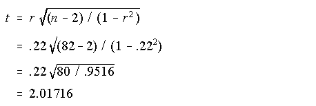
To answer this, you must calculate t as you would for the t-test:

Because the obtained value of t alternate is between 1.990 and 2.374, the probability of getting a t this large is between .05 and .02, or between 5% and 2%. This is also the probability of getting a correlation as large as .22 (or -.22) in a sample drawn from a population in which the correlation is zero.
e. What decision do you make about your hypotheses?
Because the probability is less than .05, you reject the null hypothesis.
2. Your roommate doesn't believe your conclusion, so she does her own study with a random sample of 77 students. She finds Pearson's r of 0.2203. Still using the 95% confidence level, what is the critical value?
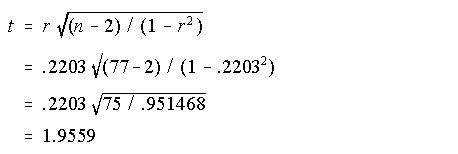
Because she has a sample of 77 students, she will have 75 degrees of freedom. Using the same 95% confidence level, the critical value of t will be between 1.994 and 1.990, the values for 70 and 80 df.
a. What are the chances of getting a correlation as large as 0.2203 in a sample of 77 students when the population correlation is zero?

Because the obtained t is smaller than 1.990, the probability of obtaining a t this large when the population correlation is zero is greater than .05.
b. What decision does she make about her hypotheses?
Because the obtained t is smaller than the critical value, she must fail to reject the null hypothesis. For her data, sampling variability could explain how she got a sample with a correlation of .2203 from a population with a correlation of zero.
3. After she finishes her study she shows you her results and says that your results are wrong. You show her your calculations and the table you used to find the critical value and convince her that your calculations were correct. You check her calculations and see that they are also correct. How do you reconcile the contradictory results?
The difference in results is due to the difference in sample sizes. While her sample correlation is a bit higher than yours, her sample is smaller, which results in a smaller value of t.
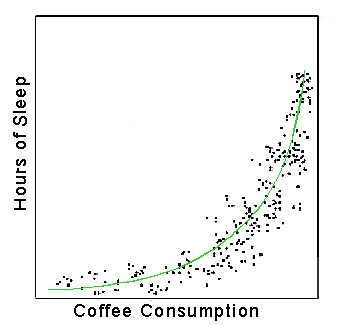
4. You don't sleep well at night, worrying about the contradiction you saw in the results of the two studies described in the preceding questions. You are so groggy in the morning that you knock your coffee cup off of the counter and it falls on the floor, spraying coffee all over the room. When you see the little brown spots scattered all over the white tile on the floor, you decide to do a scatterplot of your data and see what it looks like. You see something like the picture below.

What do you conclude after studying the scatterplot?
It appears to be the case that the relationship between coffee consumption and hours of sleep is not linear. A straight line is not a good description of the data. A curved one, like the green one drawn on the scatterplot, does a much better job of summarizing the relationship in the data.
5. Could you use Spearman's rho instead of Pearson's r? What would the effect be if you did this? Is it a good thing to do?
Yes, you could. With Spearman's rho, you are effectively calculating Pearson's r on the rank-ordered positions of the original data instead of on the original values themselves. This is why Spearman's rho is also called Spearman's rank correlation. While Pearson's r uses more of the information in the original data than Spearman's rho (because Pearson's r assumes the data is interval or ratio scaled, while Spearman's rho only expects it to be ordinal scaled), this won't be a problem here because, as you can see from the scatterplot, the relationship between coffee consumption and hours of sleep is a "monotonic" one — that is, over all parts of the range of both variables, the more coffee one consumes, the more one sleeps (!). So individuals who are near the low end of coffee consumption are also at the low end of hours of sleep and individuals at the high end of one variable are also at the high end of the other one.
6. In an attempt to develop a better understanding of your results, you do another survey. This time you ask a random sample of 90 students how long they sleep in a typical night and how many credits they are carrying. You find a correlation of .48 between hours of sleep and number of credits carried. This seems like a big difference — it's more than twice as large as 0.22 – the correlation between coffee and sleep. What would the null and alternate hypotheses be for a test of the significance of the difference?
If you only wanted to know whether the difference between the two correlations is statistically significant, your hypotheses would be:


If you wanted to know whether the correlation between sleep and credits (r =.48) was significantly higher than the correlation between coffee and sleep (r =.22), your hypotheses would be:


a. What statistical test do you use?
You would use a z-test for the difference between two Pearson's rs.
b. Using the 95% confidence level, what is the critical value?
For a two-tailed test, the 95% critical value is ± 1.96. For a one-tailed test, the 95% critical value is 1.65.
c. Perform the test. What is the probability of getting a difference between Pearson's r as large as the one between .48 and .22 (with samples of 82 and 90) when there is no difference in the population correlations? Do you reject the null?
This question wants a two-tailed test. The first step (after deciding whether it is a one- or two-tailed test and determining what the critical value is) is to use Table 5 (Fisher's r to Z) to transform the two Pearson's r values into Fisher's Z values. Note that these will not be z-scores! Table 5 gives Z = .224 for r = .22 and for r=.48, it gives Z = .523. It is the difference between .523 and .224 that are used in the actual test.
The next step is to compute the standard error of the difference between two Zs:

Finally, you calculate z:

and compare the result to the critical value, 1.96. You see, probably sadly, that the obtained z of 1.924 is smaller than the critical value, so you fail to reject the null hypothesis.
d. What do you conclude about the relative strength of associations between coffee and sleep and between credits and sleep?
Since you failed to reject the null hypothesis, you must conclude that the difference may be due to sampling variability. At this point you will probably be sorely tempted to do a one-tailed test instead of the two-tailed one. Rather than asking "is the difference between the two correlations significant" you would want to ask "is the correlation between sleep and credits (r =.48) significantly higher than the correlation between coffee and sleep (r =.22)?" The only difference in the test is that the critical value of z would be 1.65 instead of 1.96, and that for the one-tailed test the obtained z of 1.924 is larger than the critical value and you would reject the null hypothesis. It doesn't matter how badly you want to get a significant finding, though, because it is cheating to look at the result of one test and then change the hypotheses so you can do another test whose result you like better. Doing this is like asking the judge at the high jumping contest to pretend that you were really only trying to jump over the four foot bar and not the five foot one that you failed to clear.
