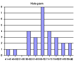
1. Prepare a table showing the frequencies, percentages, and cumulative percentages for the following data. Make the bins 5 units wide and make the first bin have the lower limit of 41.
89, 69, 76, 88, 74, 41, 49, 68, 72, 83, 66, 69, 70, 77,
56, 61, 58, 56, 63, 61, 66, 74, 69, 76, 68, 72, 83, 56
| Value | Frequency | Percent | Cum. Percent |
| 41-45 | 1 | 3.57% | 3.57% |
| 46-50 | 1 | 3.57% | 7.14% |
| 51-55 | 0 | 0.00% | 7.14% |
| 56-60 | 4 | 14.29% | 21.43% |
| 61-65 | 3 | 10.71% | 32.14% |
| 66-70 | 8 | 28.57% | 60.71% |
| 71-75 | 4 | 14.29% | 75.00% |
| 76-80 | 3 | 10.71% | 85.71% |
| 81-85 | 2 | 7.14% | 92.86% |
| 86-90 | 2 | 7.14% | 100.00% |
| Total | 28 | 100.00% |
2. Draw a histogram for the results of #1. Make the bins 5 units wide and make the first bin have the lower limit of 41.

3. Draw histograms for the following types of distributions:
a. symmetric single-peaked
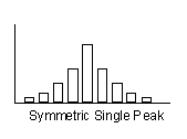
b. symmetric bimodal
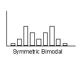
c. asymmetric single-peaked

d. asymmetric bimodal distribution
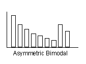
e. rectangular (flat) distribution

4. Below are the final exam scores in percentages for students in a statistics course that uses a different text.
|
|
||||||||||||||||||||||||||||||||||||||||||||||||||
a. Construct separate frequency tables for males and females. Set them up so they have 12 bins.
| Females | |||
| Value | Frequency | Percent | Cum. Percent |
| 35.00-39.99 | 0 | 0.00% | 0.00% |
| 40.00-44.99 | 1 | 4.55% | 4.55% |
| 45.00-49.99 | 0 | 0.00% | 4.55% |
| 50.00-54.99 | 1 | 4.55% | 9.09% |
| 55.00-59.99 | 0 | 0.00% | 9.09% |
| 60.00-64.99 | 1 | 4.55% | 13.64% |
| 65.00-69.99 | 3 | 13.64% | 27.27% |
| 70.00-74.99 | 4 | 18.18% | 45.45% |
| 75.00-79.99 | 1 | 4.55% | 50.00% |
| 80.00-84.99 | 4 | 18.18% | 68.18% |
| 85.00-89.99 | 4 | 18.18% | 86.36% |
| 90.00-94.99 | 3 | 13.64% | 100.00% |
| Total | 22 | 100.00% | |
| Males | |||
| Value | Frequency | Percent | Cum. Percent |
| 35.00-39.99 | 1 | 4.17% | 4.17% |
| 40.00-44.99 | 0 | 0.00% | 4.17% |
| 45.00-49.99 | 0 | 0.00% | 4.17% |
| 50.00-54.99 | 1 | 4.17% | 8.33% |
| 55.00-59.99 | 2 | 8.33% | 16.67% |
| 60.00-64.99 | 5 | 20.83% | 37.50% |
| 65.00-69.99 | 2 | 8.33% | 45.83% |
| 70.00-74.99 | 2 | 8.33% | 54.17% |
| 75.00-79.99 | 3 | 12.50% | 66.67% |
| 80.00-84.99 | 5 | 20.83% | 87.50% |
| 85.00-89.99 | 3 | 12.50% | 100.00% |
| 90.00-94.99 | 0 | 0.00% | 100.00% |
| Total | 24 | 100.00% | |
b. Draw a histogram that shows both distributions, like the one on the right side of page 58.

c. Do women do better than men? What can you say about this by examining the table and histogram you made?
d. Draw the cumulative percentage curves for the two groups on the histograms, using red for females and blue for males.

e. Locate the medians for the two groups by examining the cumulative percentage curves. What do the medians tell you in response to question 4 c?The median for females is 75.0 and the median for males is about 67.0. The females seem to have done better than the males.
f. Are either of these distributions normal? How can you tell? If they aren't, what is it about them that makes them not normal?
Neither is normal. The distribution for males is bimodal and the one for females is asymmetric and skewed.
5. Assume the mean is 72 and the standard deviation is 2.4.
a. What percent of cases lie between the mean and 2.0 standard deviations above the mean?
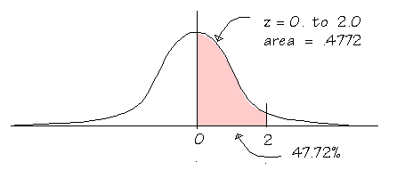
This picture shows the area between the mean (z = 0.0) and z = 2.0. You can see in the table that this area is .4772 of the total area under the normal curve. In a normal distribution, 47.72% of all cases have z-scores between 0.0 and 2.0.
| z | z to mean | smaller area | larger area |
|
|
|
|
|
|
|
|
|
|
|
|
|
|
|
|
|
|
|
|
b. What percent of cases are more than 1.8 standard deviations away from the mean?
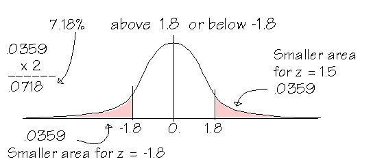
Do the right half of the distribution first. You want the ones above z =1.8, so you use the table to get the "smaller area" for z = 1.8, which is .0359. You also want the area below 1.8, which is the same as the area above z = 1.8, so you multiply .0359 by 2 and find that 7.18% are more than 1.8 standard deviations away from the mean.
| z | z to mean | smaller area | larger area |
|
|
|
|
|
|
|
|
|
|
|
|
|
|
|
|
|
|
|
|
|
|
|
|
|
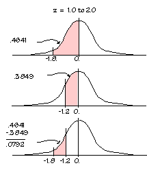
c. What percent of cases are more than 1.2 and less than 1.8 standard deviations below the mean?First convert the distances to z-scores. This is easy:
-1.2 and -1.8.
Then look for both of these on the table to get the areas. From the mean to z = 1.2 is .3849; from the mean to z = 1.8 is .4641. Subtract the first from the second:
.4641 - .3849 = .0792
to see that 7.92% of cases are between 1.2 and 1.8 standard deviations below the mean.
| z | z to mean | smaller area | larger area |
|
|
|
|
|
|
|
|
|
|
|
|
|
|
|
|
|
|
|
|
|
|
|
|
|
|
|
|
|
|
|
|
|
|
|
|
|
|
|
|
|
|
|
|
|
d. If you want the top fifteen percent of scores, how far above the mean do you have to go?
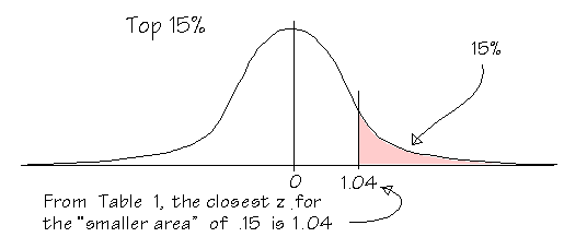
This time you start with the area (15%) and need the z-score that corresponds to it. The z-score will divide the normal curve into two sections; the smaller will be the top 15% and the larger will be the other 85%. So look for the number in the "smaller area" column closest to 0.15 and you see 1.04 is the best. You need to be at least 1.04 standard deviations above the mean to be in the top 15%.
| z | z to mean | smaller area | larger area |
|
|
|
|
|
|
|
|
|
|
|
|
|
|
|
|
|
|
|
|
|
|
|
|
|
|
|
|
|
|
|
|
|
|
|
6. If the scores on an exam are normally distributed, the mean exam score is 86.4, the standard deviation is 11.5, and the sample size is 500, how many people have scores above 95?
First, calculate the z-score. It would be:
95 - 86.4 = 8.6
and then:
8.6 /11.5 = .7478
The "smaller area" for z = .75 is 0.2266 or 22.66%. Finally, 22.66% of 500 is 113.3 which rounds to 113 people.
| z | z to mean | smaller area | larger area |
|
|
|
|
|
|
|
|
|
|
|
|
|
|
|
|
|
|
|
|
|
|
|
|
|
|
|
|
|
|

7. If the scores on an exam are normally distributed, the mean is 83.1, standard deviation is 13, and sample size is 600, how many people have scores between 95 and 105?
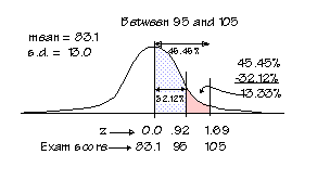
First, calculate the z-scores. For 95, it is:
(95 - 83.1) / 13 = .9154 = z
For 105, it is:
(105 - 83.1) / 13 = 1.685 = z
For raw scores of 95 and 105, the z-scores will be .9154 and 1.685. The area for z = .92 is .3212; the area for z = 1.69 is .4545, so to find the area between 95 and 105, subtract 32.12% from 45.45% to get 13.33%. To find out how many people, multiply 13.33% by 600 to get 79.98, which rounds to 80 people.
| z | z to mean | smaller area | larger area |
| : | : | : | : |
| 0.90 | 0.3159 | 0.1841 | 0.8159 |
| 0.91 | 0.3186 | 0.1814 | 0.8186 |
| 0.92 | 0.3212 | 0.1788 | 0.8212 |
| 0.93 | 0.3238 | 0.1762 | 0.8238 |
| : | : | : | : |
| 1.67 | 0.4525 | 0.0475 | 0.9525 |
| 1.68 | 0.4535 | 0.0465 | 0.9535 |
| 1.69 | 0.4545 | 0.0455 | 0.9545 |
| 1.70 | 0.4554 | 0.0446 | 0.9554 |
8. What is the z-score of the person in the 80th percentile?
This time you start with the area (80%) and need the z-score that corresponds to it. The z-score will divide the normal curve into two sections; the larger will be the bottom 80% and the smaller will be the other 20%. So look for the number in the "larger area" column closest to 0.80 and you see 0.84 is the best. You need to be at least .84 standard deviations above the mean to be in the 80th percentile or the top 20%.
| z | z to mean | smaller area | larger area |
| : | : | : | : |
| 0.83 | 0.2967 | 0.2033 | 0.7967 |
| 0.84 | 0.2995 | 0.2005 | 0.7995 |
| 0.85 | 0.3023 | 0.1977 | 0.8023 |
| 0.86 | 0.3051 | 0.1949 | 0.8051 |
| 0.87 | 0.3078 | 0.1922 | 0.8078 |
9. Does the answer to question 8 depend on the mean and standard deviation? Why or why not?
10. If your z-score is 1.85, what percentile are you in?
Since the larger area for 1.85 is .9678, 96.78% of everyone else is below you. This means you are in the 97th percentile.
| z | z to mean | smaller area | larger area |
| : | : | : | : |
| 1.84 | 0.4671 | 0.0329 | 0.9671 |
| 1.85 | 0.4678 | 0.0322 | 0.9678 |
| 1.86 | 0.4686 | 0.0314 | 0.9686 |