Weekly commentary: MAT335 - Chaos, Fractals and Dynamics

January 21 - Self-Similarity, Fractal Dimension

Self-Similarity
The fractals we have seen so far share the property of being self-similar, i.e., that arbitrarily small pieces of them replicate the whole. Thus they are extremely complicated objects (but remember that not every self-similar object is complicated, for example a cube is self-similar but it is a very simple object). More generally, we know that many objects found in nature have a kind of self-similarity; small pieces of them look similar to the whole. Some examples are clouds, waves, ferns and cauliflowers. We call these objects fractal-like. No object in nature has infinite detail, so at some small scale even the self-similiar objects cease to be self-similar. But over a (fairly wide) range of scales they are self-similar. We say that fractals have an exact self-similarity, while fractal-like objects have a self-similarity. With fractals we can be precise about what self-similarity means: the object contains small pieces that exactly reproduce the whole object when magnified. This is not necessarily true for the fractal-like objects. For them, pieces are similar to the whole when magnified appropriately. Similar meaning they 'look the same'. We recognize a cauliflower even though no two are exactly alike. This is the similarity we mean when we say that a cauliflower is self-similar: a small piece of it looks like some cauliflower. For fractals it is different. There is only one Sierpinsky triangle, and small pieces of it are Sierpinsky triangles themselves.

Fractal Dimension
The fractal dimension measures a qualitative feature of a geometric object. We can use it to distinguish different fractals (though not always; some fractals that look very different may have the same fractal dimension). We saw different types of Sierpinsky fractals (one made of triangles, one made of squares) and different types of Koch curves (one made of triangles and one made of squares). And we saw that the fractal dimension was different between the types. So although these objects were produced by a similar procedure, the result was a more 'complicated' object for one procedure than for another. The fractal dimension measured this difference in complexity. (Recall that the fractal dimension for the Sierpinsky triangle is 1.585, for the Sierpinsky square 1.892, for the Koch curve 1.262, and for the square Koch curve 1.465.) For regular objects, the fractal dimension is an integer and agrees with the usual notion of (topological) dimension. But fractals, and fractal-like objects, can have fractal dimensions that are non-integer (in fact, Mandelbrot defines a fractal as any object whose fractal dimension is not an integer; see Chapter 3 of his book).

For fractals we defined the self-similar dimension (which is the same as the fractal dimension) by covering the fractal with small pieces that are replicas of itself and counting how many of these we need as the size of the pieces tend to zero. For fractal-like objects, i.e., for self-similar objects, we used the covering dimension to measure their fractal dimension. That is, we covered them with discs (if the object sits in the plane) or balls (if the object sits in three-dimensional space) and let the diameter of the discs or balls tend to zero. We saw that the covering dimension agrees with the self-similar dimension for fractals. Measuring the covering dimension of an object (and hence measuring the fractal dimension of an object) can be effectively carried out in practice using the box-counting method (described in section 4.4 of the text).

The fractal dimension measures the 'complexity' of an object. Thus, the Koch curve has a fractal dimension greater than 1 because it is more 'complex' than a regular curve. More precisely, the number of small discs needed to cover the Koch curve increases at a faster rate as the size of the discs decrease than compared to a regular curve. This is because at smaller and smaller scales we see more and more 'wrinkles' in the Koch curve and so we need more and more discs to cover it, while a regular curve looks more and more like a straight line at smaller scales and so not so many discs are needed to cover it. The square Koch curve has a fractal dimension greater than the triangular Koch curve because it is a more complicated curve (it has more 'wrinkles' due to the fact that adding squares adds three sides while adding triangles adds only two sides to the curve in each stage of the construction). 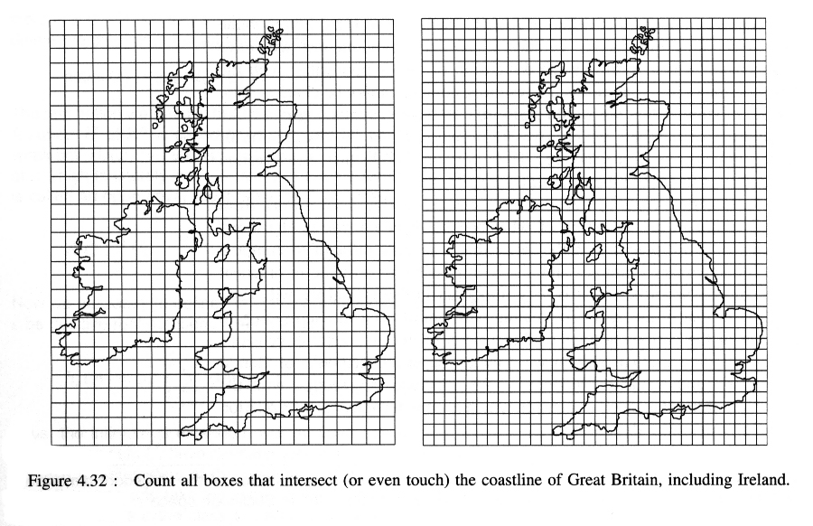For fractal-like objects like coastlines, we can use the fractal dimension to distinguish qualitatively different coastlines. For example, in your homework you would have found that the fractal dimension (D = d + 1) of the coast of Britain is greater than the fractal dimension of the coast of Spain. And this agrees with the impression we get from our eyes; the coast of Britain is more complicated that the coast of Spain.

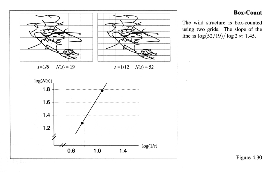
One very practical way of measuring the fractal dimension of an object is the box counting method. Here one overlays grids of boxes (in one dimension, or cubes in three dimensions) on the object and counts how many boxes intersect the object. PLotting the number N(s) of boxes intersecting the object at scale s and measuring the slope of the best-fit straight line gives an approximation to the fractal dimension of the object (see section 4.4 of the text). ( Larger view of 4.32, Larger view of 4.30.)

References

• Section 3.1 of the text (self-similarity)
• Section 4.2 of the text (measuring the lengths of curves and the exponent d; this is related to the fractal dimension of the curve - see January 14 comments)
• Section 4.3 of the text (self-similar dimension)
• Section 2.6 of the text (topological and covering dimensions)
• Chapters 2 and 3 of Mandelbrot's book; fractals in nature and fractal dimension)