Weekly commentary: MAT335 - Chaos,
Fractals and Dynamics
Top ,
Previous (Graphical analysis, bifurcations, Universality),
Next (Julia sets)
March 21
Two Dimensional Discrete Dynamical Systems
A two dimensional discrete dynamical system is defined by a function
H(x,y) of two variables (x,y). The orbits of H are the sequences
{(x_0,y_0), H(x_0,y_0), H^2(x_0,y_0), ... } . Here, (x_0,y_0) is
the initial point of the orbit, which is obtained by iterating the
function H just as we did for one dimensional discrete systems like the
logistic function. In the two dimensional case it is convenient and
informative to plot the orbits on the x,y-plane. Fixed points and periodic
points are defined the same as in the one dimensional case: p is a
fixed point of H if H(p) = p, and q is a periodic point of H of period
k if H^k(q) = q (Here I am writing p and q as two dimensional vectors, and
as usual H^k denotes the k-fold convolution of H with itself,
not the product).
The simplest two dimensional systems are the linear and affine ones. A
linear dynamical system is one of the form H(z) = Az where
A is a 2 by 2
matrix (and z denotes a two dimensional vector). An affine system is one
of the form H(z) = Az + v, where v is some vector.
0 is always a fixed point
of a linear system (but not of an affine system). Here are
some examples of linear
systems.
- A is diagonal with entries a,a.
If 0
- A is rotation about the origin. Here all orbits lie on circles
centred about (0,0).
- H(z) = v. Here all orbits move along straight lines parallel to the
vector v and passing through the initial point of the orbit (this kind of
transformation is called a "translation").
An invariant set for H is a subset B of the x,y-plane that has
the property; H(B) is contained in B. In other words, if z is in B, then
H(z) is in B too, and so the entire orbit of z is in B.
Some examples of invariants sets; any fixed point and any orbit are invariant
sets. If H(z) = Az where A is a rotation, then any circle centred
at the origin is an invariant set. If H(z) = v (translation), then any line
parallel to v is an invariant set for H.
For any invariant set B of H, we define the basin of attraction of B
to be the set W(B) = { z such that H^n(z) approaches B as n tends to
infinity}. W(B) is also called the stable set of B. Going back to
the examples above, if H(z) = Az where A is diagonal with
entries a,a, in the case 0< a <1,
W(0,0) is the whole x,y-plane,
while in the case 1 < a, W(0,0) is just (0,0).
To describe the dynamics of a two dimensional dynamical system (or a dynamical
system of any dimension for that matter), one looks for the invariant sets
and their stable sets (or at least tries to!). This information goes a long
way towards a complete description of the dynamics (i.e., of the behavior
of the orbits).
The Henon Map (pages 659 - 671)
The Henon map is a two dimensional discrete dynamical system proposed by
M. Henon in 1976 as a model for chaotic behavior in two dimensions.
Here the function H(x,y) is nonlinear (linear systems are quite easily
understandable). The function is defined by
H(x,y) = (y+1-ax^2, bx). Here, a and b are parameters;
adjusting them will change the dynamics (orbits) of H (we will usually be
interested in the case a = 1.4 and b = 0.3).
 (
Larger view . This image from Chaos and Fractals, New
Frontiers of Science by H.-O. Peitgen, H. Jurgens, and D. Saupe.
Springer-Verlag 1992.)
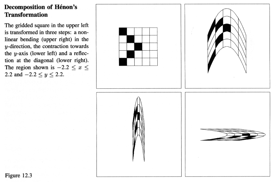
To get
an idea of what H does to points, it is worth noting that H is can be
written as a composition of 3 transformations; a bending, a compression
in the x-direction, and a reflection through the diagonal y = x (see page
662). It is this 'stretch-and-fold' action of H (for certain parameter
values) that makes this map chaotic (as we'll discuss below).
(
Larger view . This image from Chaos and Fractals, New
Frontiers of Science by H.-O. Peitgen, H. Jurgens, and D. Saupe.
Springer-Verlag 1992.)
To get
an idea of what H does to points, it is worth noting that H is can be
written as a composition of 3 transformations; a bending, a compression
in the x-direction, and a reflection through the diagonal y = x (see page
662). It is this 'stretch-and-fold' action of H (for certain parameter
values) that makes this map chaotic (as we'll discuss below).
As is usual in the study of a dynamical system we begin by looking for
periodic orbits (including the fixed points).
Fixed points and periodic points of H are points (x,y) that
solve the equations H^k(z) = z for some k (note that this denotes k-fold
composition of H, not the product).
We find that for a < (b-1)/4,
there are no fixed points. If a = (b-1)/4 there is one fixed
point (2/(b-1), 2b/(b-1), and if (b-1)/4 < a there are two
fixed points p_1 and p_2. As the parameter a is increased a
sequence of period doubling bifurcations occur. Here too we see
Universality: the rate at which the bifurcations occur is given by the
Feigenbaum constant 4.669... . The period doubling "cascade" is
completed when a reaches the value 1.05 (see Figure 12.15).
As in the case of the logistic equation, the period doubling signals the
onset of chaos. For parameter values a > 1.05 and b = 0.3,
the Henon map
possesses an invariant set A situated near the origin.
 (
Larger view.)
The dynamics on this attractor A is chaotic. That is, points
move around the attractor in an apparently random fashion. More
precisely, the dynamics of the Henon map on the attractor exhibits the hall
marks of chaos: sensitive dependence on initial data, periodic points
are everywhere, and there are ergodic orbits (i.e., orbits that visit every
neighborhood of the attractor). However, we still lack a
mathematical proof that the
dynamics on the attractor is chaotic.
(See the
Henon applet to see the dynamics on the attractor.)
(
Larger view.)
The dynamics on this attractor A is chaotic. That is, points
move around the attractor in an apparently random fashion. More
precisely, the dynamics of the Henon map on the attractor exhibits the hall
marks of chaos: sensitive dependence on initial data, periodic points
are everywhere, and there are ergodic orbits (i.e., orbits that visit every
neighborhood of the attractor). However, we still lack a
mathematical proof that the
dynamics on the attractor is chaotic.
(See the
Henon applet to see the dynamics on the attractor.)
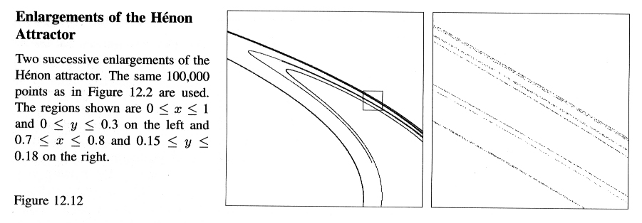
Another feature of the Henon attractor is that it has a fractal-like structure.
From afar it looks like a long winding curve,
but when you zoom in on a small piece
the curve breaks into several thinner strands close together.
 (
Larger view.)
And when you
zoom in to one of these smaller strands it too breaks apart into several
thinner strands, etc; see Figure 12.12. In fact, one can measure the fractal
dimension of the attractor (via the box counting method); it is approximately
1.3 (see page 670). It is this fractal-like structure of the attractor
which makes it "strange". If you looked at the attractor for other parameter
values (for some parameter values there is no attractor though), it may
appear either as a finite set of points (eg., an unstable periodic orbit)
or as a solid region (eg., the stable set of a stable periodic orbit) - these
attractors are not "strange", and the dynamics on them is not chaotic.
(
Larger view.)
And when you
zoom in to one of these smaller strands it too breaks apart into several
thinner strands, etc; see Figure 12.12. In fact, one can measure the fractal
dimension of the attractor (via the box counting method); it is approximately
1.3 (see page 670). It is this fractal-like structure of the attractor
which makes it "strange". If you looked at the attractor for other parameter
values (for some parameter values there is no attractor though), it may
appear either as a finite set of points (eg., an unstable periodic orbit)
or as a solid region (eg., the stable set of a stable periodic orbit) - these
attractors are not "strange", and the dynamics on them is not chaotic.
It is the "strangeness" of the strange attractor which makes the dynamics
of the Henon map chaotic. Recall that starting with an arbitrary point in
the plane, the orbit of that point under iteration by the Henon map will
either move outwards to infinity or else will move towards the attractor.
In the former case the dynamics is simple (the orbit goes to infinity). In the
latter case the orbit becomes quite complicated as it converges to the
attractor. When it is very close to the attractor (which doesn't take too
long; convergence of orbits to the attractor is exponentially fast, i.e.,
the distance between points in the orbit and the attractor diminishes
like c*e^n for some c > 0 and n < 0), the orbit moves very much like an
orbit on the attractor. So there are two types of behavior of this system;
one is very regular and the other is chaotic. If it is to model some physical
phenomena, then the orbits that go off to infinity are not relevant and
what we discover then is that a relatively simple model produces an
extremely complicated dynamics. In the years prior to the creation of the
"strange attractor" paradigm, if a scientist observed chaotic behavior
in his model or experiment he would most likely ascribe it to an incorrect
mathematical model of the phenomena or else to errors in the experiment
(see David Ruelle's book for his comments about this). Now it is accepted
that simple models can be intrinsically complicated to an infinite degree
and part of the "boom" in chaos theory were the countless discoveries of
chaos in many standard mathematical models that hitherto had not been suspected
of producing anything "unpredictable" or "uncontrollable".
Later sections of Chapter 12 describe some of the quantitative measurements
one can make of chaotic dynamics such as the Lyapunov exponents (Section
12.5) and reconstruction of strange attractors from experimental data
(Section 12.7).
Top ,
Previous (Graphical analysis, bifurcations, Universality),
Next (Julia sets)