MAT 335 Project
Fractal Landscapes
Min-Fang Grace Tsai
for
Dr. Randall Pyke
May, 2003
Table of Contents
I. Introduction…………………………………………………………..3
II. Midpoint Displacement Method……………………………………4
Important Parameters……………………………………6
III. Fractal Terrain Applet…………………………………………….8
Basic Algorithm…………………………………………...8
Basic Controls……………………………………………..9
Render As: Three Views………………………………...10
Parameters……………………………………………….12
IV. Cloud Applet………………………………………………………20
Basic Algorithm………………………………………….20
Parameters……………………………………………….21
V. Random Number Distribution…………………………………….28
Distribution
Functions…………………………………..28
Mean and Variance……………………………………...33
VI. More Realistic Clouds
(3D Spherical Cloud)……………………37
VII. Conclusion………………………………………………………..38
VIII. References……………………………………………………….39
I. Introduction
In nature, many
fundamental geometrical shapes contain self-similar structures. For living
organisms, this self-similarity ensures their survival. For example, plants have
a branching structure that allows the capture of maximum sun light, and blood
vessel systems in lungs have a similar structure to allow maximum amount of
oxygen. Individual islands, mountains, coastlines, and rivers all display
self-similarity as well. Therefore, a reasonable course of action is to model
real-world objects using the principles of fractal self-similarity. Some
natural objects can be modeled by deterministic classical fractals, such as the
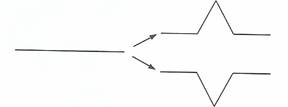
If the orientations are chosen at random in each replacement step, the resulting image is the random Koch curve. An “island” can then be constructed by linking three different versions of the random Koch curve into a random Koch snowflake, as shown below:
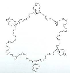
However, as we can see, the result is not very realistic. First, this report will introduce another method: the midpoint displacement method, in generating fractal landscapes and clouds, followed by an explanation of the different computer programs used. Then, it will describe the relationships and effects of the different parameters in generating various images.
II. Midpoint
Displacement Method
A natural extension of the von Koch construction is the midpoint displacement method. Random midpoint displacement is a recursive generating technique that was applied to normal Brownian motion as early as the 1920’s by N. Wiener. Later, its use in computer graphics has been widely popularized by Fournier, Fussell, and Carpenter in areas such as fractal landscape and clouds.
To understand the algorithm of midpoint displacement method, first consider a square grid on the x-z plane. The algorithm can be summarized below:
1) split the square up into a 2*2 grid
2) vertically displace each of the 5 new vertices by a random amount in the y-direction
3) repeat this process for each of the new squares, decreasing the displacement for each iteration
Graphically, it can be conceptualized as follows:
As the iterations grow, the landscape would evolve in the following manner:
Note that for smaller iterations, the displacements seem to be larger than for larger iterations. Or, in other words, the peaks are higher and the valleys are deeper.
The displacement at each iteration is:
Displacement amount = avg +
scale*random
Where the avg is average value of the adjacent corners,
and random is the random number. Scale usually decreases at a
rate of 1/2H, where H is related to roughness. More will be said
about the roughness parameter later.
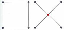
The construction of the square grids can be broken down into two refinement steps. First, for all squares, the surface heights over the midpoints are computed by interpolation from the heights of their four neighbouring points, followed by a random offset. In the diagram below, the four neighbouring points are shown by gray dots, while the new midpoint is shown by red.
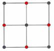
In the following step, the elevations of the remaining intermediate points are computed. When the first step has been carried out, these points should also have three neighbour points on the base square, and four neighbour points on following iterations. Again, the new points are shown in red.
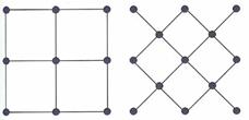
This next diagram shows the grid construction for the next iteration, iteration=2:
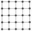
For k iterations, there are 2k squares on each side, and therefore the whole area would have 2k ´ 2k small squares. The number of vertices on each side can be represented by a geometrical series: 2+(20+21+…+2k-1). Refer to the diagrams of landscapes with different iterations on the last page (p.2) for more examples.
Important Parameters
Finally, some important parameters to this algorithm are discussed briefly.
Random Number
To generate a random number, the computer uses
a function called “random number generator.” The input to the generator is
known as a “seed,” and the output is a random number. With the same “seed,” the
generator would generate the same random number, and hence, the same landscape.
Varying the seed would vary the landscape. Also, the random number generator
normally follows a normal random distribution function, with mean m= 0 and variance s2=1. A different
distribution function, or a different mean or variance would generate different
random numbers, and thus different landscapes.
Roughness/Scale
Roughness is the factor by which the
perturbations are reduced on each iteration. Usually,
a factor of 2 is the default, and higher values result in a smoother surface
while lower values result in a rougher surface. Roughness also is related to
scale:
scale = 1/2roughness
Thus, a larger scale means a smaller roughness
value, and a rougher landscape. And vice versa.
Initial Points
It is desirable to specify some initial points,
normally on the corners of the initial rectangles. This provides some degree of
control over the macro appearance of the landscape.
Sea Level
The sea “floods” the terrain to a particular
level simulating the water level. The terrain that is below the sea level is
simply covered up in water and cannot be seen.
Color Ramp
The terrain surface is shaded in color based on
the height. Normally two or three colors are defined for particular heights,
for example, at the sea surface it is usually blue, and nearer to the mountain
peaks it is white.
Number of Iterations
At k iterations, there will be 2k ´ 2k small square mesh. Therefore, the larger the number of iterations means the smaller the squares on the grid. It results in the density of the mesh that results from the iteration process.
Grid Type
The type of grid that is discussed above is a square grid. Usually a square grid is used for its simplicity. However, we can vary the grid to other geometrical shapes, like a triangle or a hexagon, as shown in the following diagram.
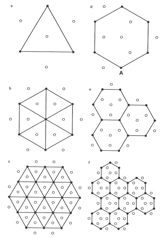
Triangular (left) versus hexagonal (right) tiles and midpoint displacements
III. Fractal Terrain Applet
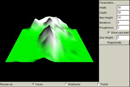
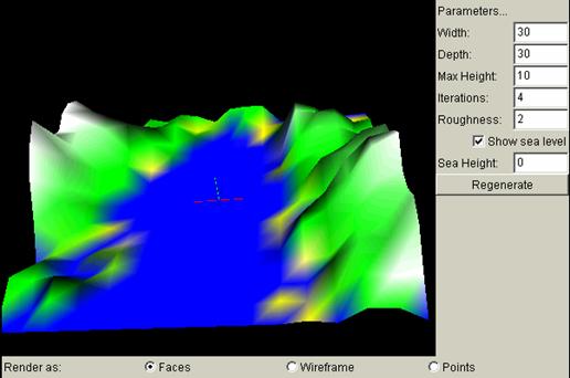
I have provided
a program that draws the fractal terrain using midpoint displacement method
described above. Below is a screen snapshot.
Basic Algorithm
It is basically the same as the midpoint displacement method described above. However, at each stage of the displacement, the scale does not decrease with the increase of the number of iterations. Also, the sign of the displacements is random, and is generated with another random number. There are two components in a displacement: the absolute value of displacement and its sign of displacement. The height of the midpoint is calculated as the average of the neighbouring heights, multiplied by a random number and a random displacement sign.
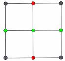
For even rows, simply copy the existing row and add new points, as shown in red dots in the below diagram. For odd rows, insert a whole new row between the two old rows, as shown in green dots.
Basic Controls
Draw new fractal – Click on Regenerate button
Rotate – click and hold on the graph with the left mouse button, and drag the graph to a desired orientation.
Zoom in/out – press Alt key on the keyboard, and click and hold the left mouse button at the same time. To zoom out, drag the graph towards you and “outwards” from the screen. To zoom in, drag the graph away from you and “into” the screen.
Below is a diagram of the axis that is visible on the applet. Using these three coloured axes, users can identify the orientation of the fractal terrain.
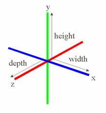
A 3D object inside the computer can be specified by three values: width in the x direction, depth in the z direction, and height in the y direction. The height and width of the computer screen corresponds to the x-y plane. The fractal landscape is constructed as thus: the x-z plane is in the orientation of the square grids, and the vertical displacements are made in the y direction.
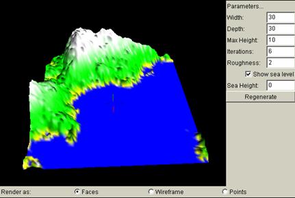
Render As: Three Views
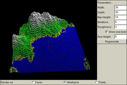
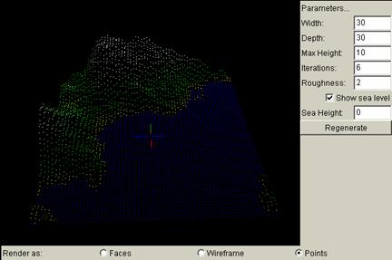
At the bottom of the applet, there are three options to choose from: faces, wireframe, and points. They represent three different views of the same terrain landscape. Faces show the landscape as if in nature, where the terrain is a smooth surface with differing colours. Wireframe shows the landscape as grid mesh, and is most suitable when showing grid constructions with each iteration. Points show the vertices of these square lattices. They are more apparent for high iterations, and lower iterations may not seem apparent enough. Below are the three different views using the same landscape:
Faces View:
Wireframe View:
Points View:
Parameters…
The parameters available on the right side of the applet are explained below with corresponding screen shots showing different values. Most are shown with the faces view, except for iterations. Note that since all graphs are generated randomly, the shapes are not the same, and the examples are just for demonstrative purposes.
Width
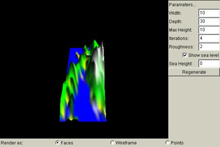
Changing the width on the applet would change the strip of terrain to be broader/narrower in the x direction, as is demonstrated in the below screen shots.
Width = 30
Width = 10
Depth
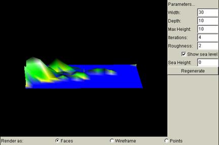
Changing the width on the applet would change the strip of terrain to be broader/narrower in the y direction, as is demonstrated in the below screen shots.
Depth = 30
Depth = 10
Max Height
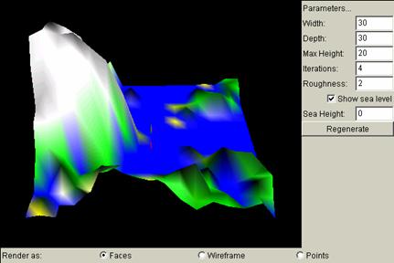
Maximum height denotes the maximum of the height of the mountain peaks. It sets the upper boundary for the range of values. The larger the value, the higher the highest peaks.
Max Height = 10:
Max Height = 20:
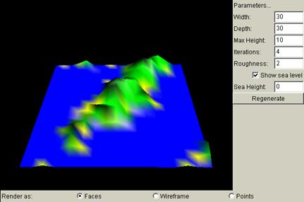
Iterations
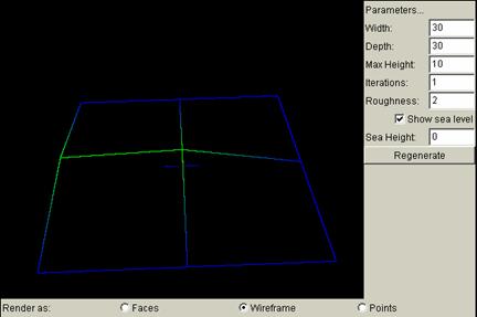
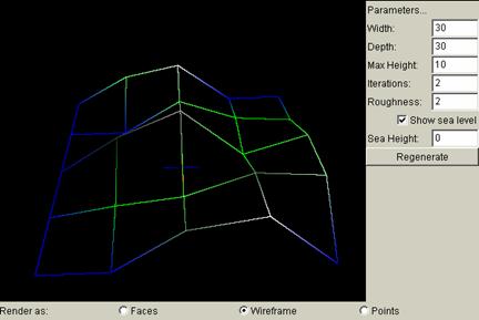
Iterations is related to how dense the square grids are. For an iteration of k, there are 2k squares for each side of the original grid. The larger the iterations, the denser the grids. In order to show more clearly how the number of iterations changes the grids, and how the grids are constructed, the following terrain views are captured under wireframe.
Iterations = 1:
Iterations = 2:
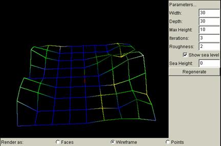
Iterations = 3:
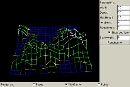
Iterations = 4:
Roughness
Roughness is the factor by which the
perturbations are reduced on each iteration. A
smoother surface has a higher value, and a rougher surface has a lower surface.
Below are some examples showing its significance.
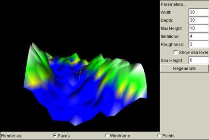
Roughness = 2:
Roughness = 5:
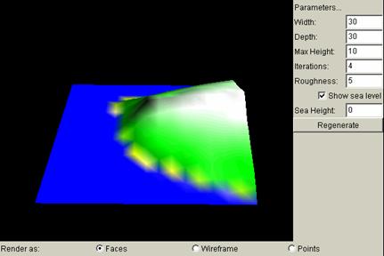
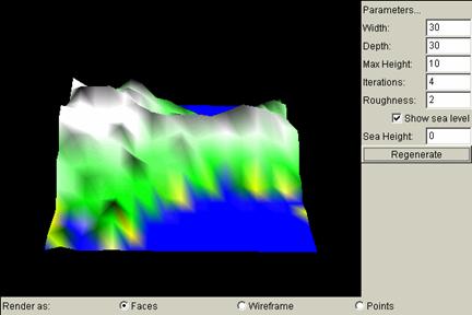
Show Sea Level
The sea “fills” up the terrain to the sea level, leaving everything under the level invisible. Everything underneath will just be covered up with a smooth surface. Putting a check mark in the box indicates showing the sea level and filling up the sea, while not putting a check indicates showing the terrain below the sea level.
With Sea Level:
Without Sea Level:
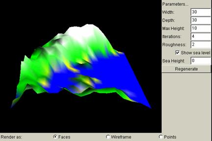
Sea Height
This determines the height to which the sea will be filled up to. Note that because of the colouring scheme, all heights lower than or equal to 0 are coloured blue, and heights above 0 are coloured green. Therefore, for a sea level of higher than 0, the terrain will be more like a plateau rather than a sea, as is shown in the below diagram. For a terrain with sea level of lower than 0, the graphs would not appear drastically different since the fill-up colour is also blue, the default. Thus it will not be shown here.
Sea Height = 0:
Sea Height = 2: