IV

IV. Cloud Applet

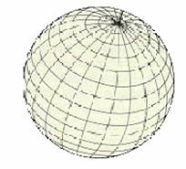
The cloud applet is a program I have provided that models the real-world clouds. Below is a screen snapshot.

Basic Algorithm

This algorithm is similar to the above fractal terrain algorithm in that they both use the midpoint displacement method. However, instead of a vertical height displacement, the height is mapped to a corresponding colour. The lowest valleys correspond to black areas, and the highest peaks correspond to white areas. The final cloud is thus a top view of the “landscape” where the height now defines the shade of gray to be used. Each vertex on the square grid will correspond to one pixel on the applet. Width and depth of the graph area are now dependent on the number of iterations, and not user-defined. For k iterations,

Width*Depth of the terrain

= the number of points on the grid

= number of pixels on the applet

= [ 2+(2⁰+2¹+…+2^k-1)] ²

Therefore, with only a few iterations, there will only be a small number of pixels, and the graph area would be very small.

Parameters…

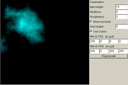
The parameters available on the right side of the applet are explained below with corresponding screen shots showing different values. Note that since all graphs are generated randomly, the shapes are not the same, and the examples are just for demonstrative purposes.

Max Height

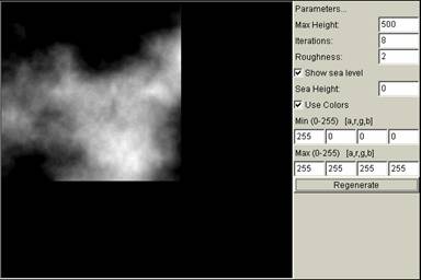
It is the maximum intensity of “whiteness.” In theory, the larger the value of maximum height, the “whiter” the cloud. However, because all clouds are coloured white after a certain height, the difference is not very obvious. Thus, a more drastic example is taken. It can be seen that with a larger max height, the cloud seems “purer” and “whiter,” with less areas of “gray.”

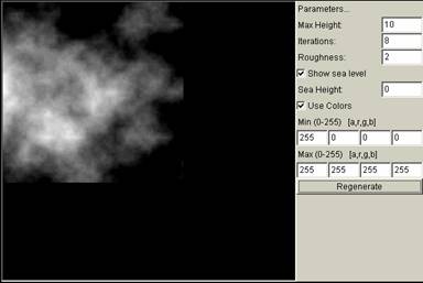
Max Height = 10:

Max Height = 500:

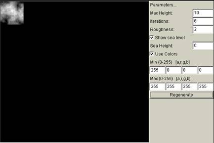
Iterations

As stated above, iterations changes the number of vertices on the grid, and so in turn changes the number of pixels used to draw this graph. A larger value for iterations means a larger graph area, while a smaller value means a smaller graph area. Note that iterations above 10 requires really complex computation and this applet may not work.

Iterations = 8:

Iterations = 6:

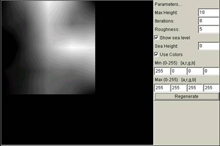
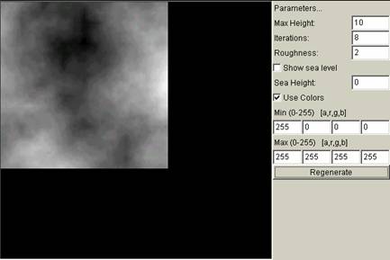
Roughness

The smaller the value, the rougher the cloud looks, with more definite “edge” to the cloud. The larger the roughness value, the smoother the cloud looks, where the white just gradually diminishes into black.

Roughness = 2:

Roughness = 5:

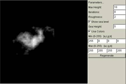
Show Sea Level

This determines whether or not to cover all the lower heights under a colour coating of black. With the sea level, less of the clouds can be seen. Without the sea level, more of the clouds can be seen, in the colour gray around the edges. More black areas are filled with gray clouds.

With Sea Level:

Without Sea Level:

Sea Height

This changes the sea level height. The lower the height, the larger the cloud and the more gray areas. With a larger height value, less of the clouds is shown, and the less gray areas.

Sea Height = 0:

Sea Height = 5:

Use Colors

This checkmark checks off whether the user wishes to see the clouds in black and white. Of course, for white clouds against a black background it does not matter, but clouds of other colors can indeed be generated by varying the next parameter values: [a,r,g,b].

Min-Max (0-255) [a,r,g,b]

This denotes the range of the colors, from the minimum to the maximum. One pixel is assigned a value for each of [a,r,g,b]. But what is [a,r,g,b]? It is a standard color scheme for computer systems called sRGB, co-developed by Microsoft and HP. They mean:

a – alpha

r – red

g – green

b – blue

Alpha is transparency. The higher the value, the greater the opacity of color, and the lower the value, the greater the transparency. Its change is hard to notice. r,g,b are intuitively easy to comprehend. All of these take on a range of values between 0-255. Check out this website to get a complete listing of [r,g,b] values for all colors.:

http://www.daveandal.com/books/7868/charting/dotnet-color-list.aspx

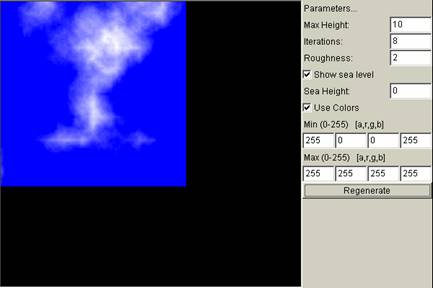
In order to change the colors of the clouds and the sky, we simply need to change the corresponding values for the range of [a,r,g,b]. Below are some experiments of the variations.

When one of the values has a range of 255-255, the background sky would change to that colour. For example, to obtain a blue sky, change the range of b to be 255-255.

Min – [255, 0, 0, 255]

Max – [255, 255, 255, 255]

To change the color of the cloud, the simplest way is to change one of the ranges to 0-0. For example, below is an example when the r value has a range of 0-0.

Min – [255, 0, 0, 0]

Max – [255, 0, 255, 255]

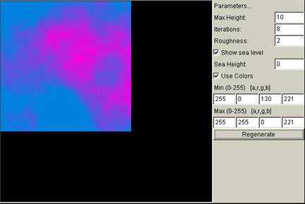
Changing several ranges, the following graph with blue background and purple clouds can be obtained.

Min – [255, 0, 130, 221]

Max – [255, 255, 0, 221]

V. Random Number Distribution

There are two ways to change the distribution of random numbers. One is to change its distribution function and one is to vary its mean or variance. The following two sections describe each change in turn. Because of the complexity of changing mathematical parameters in Java applets, I have done the following experiments using MATLAB. MATLAB is a mathematical computer program, and has a “random number generator” for different distribution functions. Special thanks to Dr. Pyke for providing the original program at this URL:

http://www.math.toronto.edu/courses/335/fractal_landscape/land.m

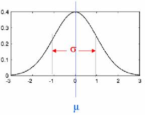
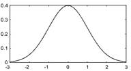
Distribution Functions

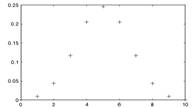
Usually, the computer calculates a random number with a normal, or Gaussian, distribution. What happens if a different distribution function is used? Below are the distribution function graphs of the normal, binomial, and gamma. All of these display a “bell-shape.” Therefore, by adjusting the distribution function to be of the same mean and variance, these three functions would look similar in both shape and values.

Normal:

Binomial: Gamma:

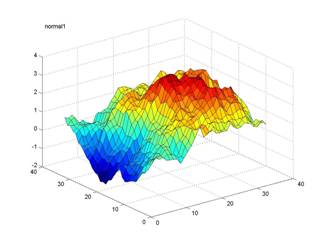
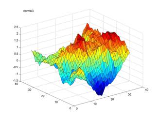
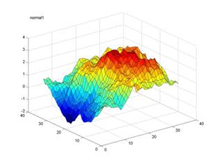
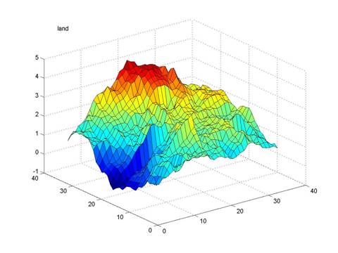
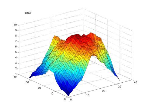
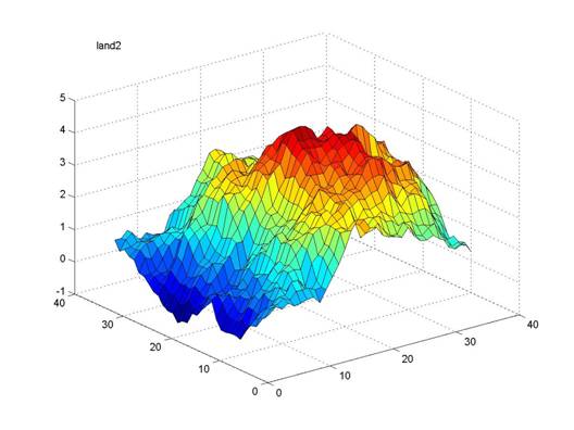
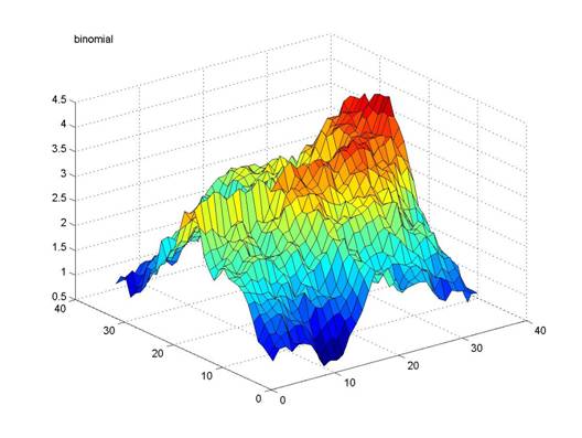
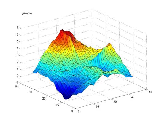
Using these distribution functions to plot fractal landscapes, all three look pretty much the same. They might as well be a family of graphs of the same distribution. Next is an experiment showing how much their fractal landscape look alike. In order to facilitate the comparisons, other parameters that might effect the appearance have been adjusted to take on the same values. I have set mean = 1, variance = 1, and the seeds rand = 10 and randn = 10.

Normal Distribution:

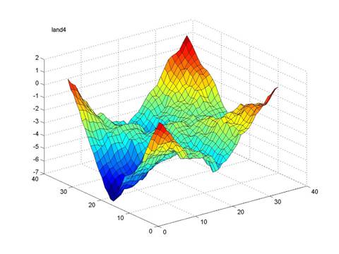
Binomial Distribution:

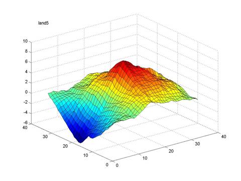
Gamma Distribution:

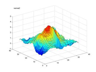
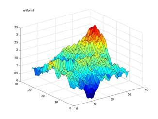
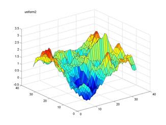
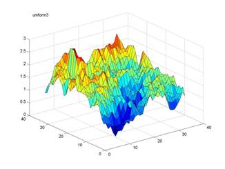
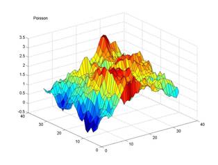
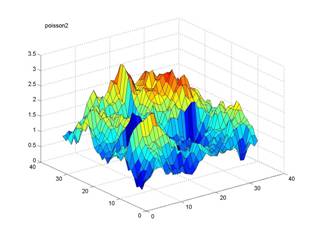
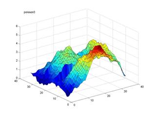
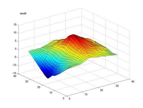
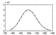
The next two distribution functions, uniform and Poisson, have distinctively different shapes from the normal distribution. Thus, in theory, landscapes using these different distributions should appear distinctly different. Uniform would result in values that are very widely spread. (ie. even chance of obtaining all values in the (0,1) range) Poisson would result in values concentrated near the lower end, or more, smaller displacements.

Normal:

Uniform: Poisson:

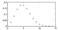
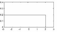
Note that, as before, I set mean=1, variance=1.

Mean and Variance

The following diagram shows the mean m and the variance s² on a distribution function.

Mean

By changing the mean, the elevation landscape can be effectively changed. A higher mean results in a higher elevation, and a lower mean results in a lower elevation, as shown in the following graphs.

m = 0, s²=1:

m = 5, s²=1:

m = -5, s²=1:

Indeed, for a higher m, the range of height is 1-10, and for a lower m, the range is (–7)–2. The elevation of the whole graph is thus changed. Note, however, that at the four corners, both graphs seem to be “tied.” This is due to the fact that these points are given fixed, initial displacements, but their have values that are “less likely to happen.” If the four initial points were not picked manually, but chosen to be values close to the mean, this “tying down” would not happen.

Variance

By changing the variance, we are effectively changing the “spread” of the values. For a larger variance, the values are more “spread out,” and there would be more extreme values, ie. more really large random numbers, and more really small random numbers. Or, in other words, more higher peaks and deeper valleys. For a smaller variance, the landscape would have less difference in height. The following three graphs are in increasing order of variance. It is clear that the range of height values becomes larger: from (-1)-5 to (-15)-15.

m = 0, s²=1:

m = 0, s²=3:

m = 0, s²=5:

VI. More Realistic Clouds (3D Spherical Cloud)

This is a topic that I have pursued in the preparations of the project, but unfortunately have no sufficient time to finish. However, since it is very interesting, so I will devote one section here to its discussion. In order to model more realistic, 3D clouds, the first thought was to use a 3D shape as the original grid, and evolve from there. A cubic square came to mind, but was later rejected. It is because that the boundaries, or the 90 degrees angles at each side, cannot be displaced or moved, and thus would not make a realistic cloud. The next was a 3D spherical cloud.

The basic algorithm for a 3D spherical cloud is the midpoint displacement method. However, instead of starting with a square grid on the x-z plane, now we start with a 3D sphere. Spherical coordinates is chosen for easy computations. Also, the grids are now constructed from longitude/latitude of the globe. Each point is randomly displaced in terms of differing radius. Or, in other words, differing in the distance to the centre of the sphere. Finally, the scaling factor would need to depend on ф, since the squares are smaller near the poles, and it is preferable to have a “flat” cloud.

However, there may be some potential problems with this model. Points on a spherical grid are not evenly distributed. Would the computer be able to draw the points near the poles? Also, with the use of pixels, this would be a 2D surface in a 3D space, but not a 3D object. Most importantly, how will it look like? Would it be a realistic cloud, or just a lump, like a rock or an asteroid?

How else could a realistic cloud be modeled with fractal images? In the real world, when one looks up into the sky, the clouds almost seem like a 2D object, with differing layers, but not necessarily a 3D object. One possible solution, then, is to start with the 3D spherical cloud construction. Next, calculate the thickness at any one particular point, and map the corresponding values to a 2D screen, which in turn determines the shape of the final cloud.

VII. Conclusion

In order to generate real-world objects, their self-similarity property makes them easy for mathematical fractals to construct. Self-similarity is sometimes apparent in appearance, but sometimes only in a statistical sense. Midpoint displacement method is an algorithm that models geometrical construction principles in nature, such as fractal terrain or fractal cloud. There are several important parameters: random number, roughness, initial points, sea level, color ramp, number of iterations, and the type of grids. A detailed discussion of the effect of each is described above, using the applet programs that I have wrote to provide concrete examples for both the landscape terrain and the clouds. A more complicated of these parameters is the random number. Two factors concerning the random number distribution are different distribution functions, and different mean and variance. They are both described thoroughly with the help of the MATLAB landscape program generously provided by Dr. Pyke. When constructing clouds, is there a way to make them more realistic? Several options of “going 3D” are proposed, such as using a 3D spherical cloud, and projecting its thickness onto a surface.

Fractal landscapes that are constructed with the above algorithms are by no means perfect, and have some major short-comings. Firstly, they fail to include river networks. Secondly, they generate unnatural features known as the “creasing problem.” Lastly, because most images are constructed with normal distribution, which has a symmetric bell shape, the valleys and mountains are also symmetric in shape. There are still many areas that open for innovative improvements.

Some real-world applications for the technology of fractal landscapes include computer graphics, and geomorphology. Computer graphics can use fractal images in creating digital pictures, or graphics and animations used in the production of film. Geomorphology can use fractal images in simulating different landscapes, or envisioning a geographical system. Both of these applications depend on the “realness” of fractal landscapes. Thus, the art of fractal landscapes is still a hot topic today.

VIII. References

Books

· Chaos and Fractals – New Frontiers of Science by Peitgen, Jurgens, and Saupe

· The Science of Fractal Images by Barnsley, Devaney, Mandelbrot, Peitgen, Saupe, and Voss

· Fundamentals of Probability by Saeed Ghahramani

URLs

Algorithms:

· http://www.math.toronto.edu/courses/335/fractal_landscape/fractal_lands.html

· http://astronomy.swin.edu.au/~pbourke/terrain/frachill/

sRGB color scheme:

· http://www.daveandal.com/books/7868/charting/dotnet-color-list.aspx

· http://www.srgb.com/index.html