Emulation/Prediction Test Problems
Uncertainty Quantification Test Problems
Multi Fidelity Simulation Test Problems
Screening Test Problems
Borehole Function
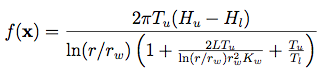
Description:
Dimensions: 8The Borehole function models water flow through a borehole. Its simplicity and quick evaluation makes it a commonly used function for testing a wide variety of methods in computer experiments.
The response is water flow rate, in m3/yr.
Input Domain and Distributions:
The input variables and their usual input ranges are:| rw ∈ [0.05, 0.15] | radius of borehole (m) |
| r ∈ [100, 50000] | radius of influence (m) |
| Tu ∈ [63070, 115600] | transmissivity of upper aquifer (m2/yr) |
| Hu ∈ [990, 1110] | potentiometric head of upper aquifer (m) |
| Tl ∈ [63.1, 116] | transmissivity of lower aquifer (m2/yr) |
| Hl ∈ [700, 820] | potentiometric head of lower aquifer (m) |
| L ∈ [1120, 1680] | length of borehole (m) |
| Kw ∈ [9855, 12045] | hydraulic conductivity of borehole (m/yr) |
For the purposes of uncertainty quantification, the distributions of the input random variables are:
| rw ~ N(μ=0.10, σ=0.0161812) |
| r ~ Lognormal(μ=7.71, σ=1.0056) |
| Tu ~ Uniform[63070, 115600] |
| Hu ~ Uniform[990, 1110] |
| Tl ~ Uniform[63.1, 116] |
| Hl ~ Uniform[700, 820] |
| L ~ Uniform[1120, 1680] |
| Kw ~ Uniform[9855, 12045] |
Above, N(μ, σ) is the Normal distribution with mean μ and variance σ2. Lognormal(μ, σ) is the Lognormal distribution of a variable, such that the natural logarithm of the variable has a N(μ, σ) distribution.
Modifications and Alternative Forms:
The range of Kw may be changed to [1500, 15 000], creating a more nonlinear and non-additive function, as in Morris et al. (1993) and Xiong et al. (2013).In the context of emulating computer models with both quantitative and qualitative factors, Zhou et al. (2011) use the qualitative factors z1 = r, z2 = Hu–Hl and z3 = Kw, each at three levels. The remaining four variables are used as quantitative factors.
For the purpose of input variable screening, Moon (2010) and Moon et al. (2012) add 12 inert input variables.
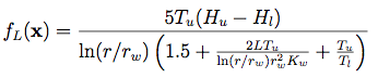
For the purpose of multi-fidelity simulation, Xiong et al. (2013) use the following function for the lower fidelity code:
Code:
R Implementation
MATLAB Implementation, Lower Fidelity
R Implementation, Lower Fidelity
References:
An, J., & Owen, A. (2001). Quasi-regression. Journal of Complexity, 17(4), 588-607.
Gramacy, R. B., & Lian, H. (2012). Gaussian process single-index models as emulators for computer experiments. Technometrics, 54(1), 30-41.
Harper, W. V., & Gupta, S. K. (1983). Sensitivity/uncertainty analysis of a borehole scenario comparing Latin Hypercube Sampling and deterministic sensitivity approaches (No. BMI/ONWI-516). Battelle Memorial Inst., Columbus, OH (USA). Office of Nuclear Waste Isolation.
Joseph, V. R., Hung, Y., & Sudjianto, A. (2008). Blind kriging: A new method for developing metamodels. Journal of mechanical design, 130, 031102.
Moon, H. (2010). Design and Analysis of Computer Experiments for Screening Input Variables (Doctoral dissertation, Ohio State University).
Moon, H., Dean, A. M., & Santner, T. J. (2012). Two-stage sensitivity-based group screening in computer experiments. Technometrics, 54(4), 376-387.
Morris, M. D., Mitchell, T. J., & Ylvisaker, D. (1993). Bayesian design and analysis of computer experiments: use of derivatives in surface prediction. Technometrics, 35(3), 243-255.
Xiong, S., Qian, P. Z., & Wu, C. J. (2013). Sequential design and analysis of high-accuracy and low-accuracy computer codes. Technometrics, 55(1), 37-46.
Worley, B. A. (1987). Deterministic uncertainty analysis (No. CONF-871101-30). Oak Ridge National Lab., TN (USA).
Zhou, Q., Qian, P. Z., & Zhou, S. (2011). A simple approach to emulation for computer models with qualitative and quantitative factors. Technometrics, 53(3).
For questions or comments, please email Derek Bingham at: dbingham@stat.sfu.ca.