Learning: Supervised, Unsupervised, and Reinforcement

Introduction to Supervised Learning

the task of supervised learning is as follows:

Given a training set of N example input-output pairs

\((x_1,y_1), (x_2,y_2), \ldots (x_N,y_N)\)

where each \(y_i\) was generated by an unknown function \(y = f(x)\), discover a function \(h\) that approximates the true function \(f\)

\(x\) and \(y\) can by any type of value, not just numbers

the function \(h\) is called the hypothesis

a learning algorithm can be thought of as searching through the space of hypotheses for a hypothesis function that works well on the training set, and also on new examples that it hasn’t seen yet

to test the accuracy of the hypothesis, a set of test examples (different from the training set) is used

• in practice, you typically have one large test set of data to work with, and so you split this data into a training set and a test set
• a split of 80% for the training set and 20% for the test set is a common split

we want to find a hypothesis function that generalizes well, i.e. that accurately predicts the outcome of examples it hasn’t seen before

if the output values \(y\) are numbers, we call the problem a regression problem

if instead the output values are a small set of values (like ham/spam, or sunny/cloudy/rainy), then we call it a classification problem

there are different ways to approach supervised learning, and here we will look at three common ways of doing it

• decision trees
• regression
• k-nearest neighbor

Decision Trees

a decision tree is a tree structure where each node corresponds to a question, and each child of the node corresponds to an answer to the question

starting at the root, a decision tree leads you through a series of questions that, when it hits a leaf node, will hopefully give you a good answer to the overall question the tree was designed to answer

given labeled data, relatively small decision trees can be efficiently learned in many cases

• they are one of the standard ML techniques that people reach for in practice
• random forests are a sort of generalization of decisions trees that are quite popular in practice

following the main example in the textbook, suppose we want to learn a decision tree about whether or not we would wait for a table in a restaurant

features to be considered are things like:

• alternate: is there another restaurant nearby?
• bar: is their a comfortable waiting area?
• Friday/Saturday: is it Friday or Saturday? this is a yes/no feature
• Hungry: yes/no are you hungry?
• Patrons: how many people are currently in the restaurant: none, some, full?
• Price: is the restaurants price low, medium, or high?
• Raining: is it raining outside?
• Reservation: do we have a reservation?
• Type: what kind of food: French, Italian, Thai, or burger?
• Wait time: estimated waiting time according to restaurant: 0-10min, 10-30min, 30-60min, >60min

note that the numeric values have been reduced to small finite sets of values

here is some example data:

this isn’t a lot of data, but it is just a small example that can be checked by hand

here is an example of a decision tree that one could use to make a decision about where to eat:

you start at the top and follow the nodes downwards, taking the path according to your answers for each of the questions in the node

for many applications, a decision tree is a pretty good way of making decisions or predictions

it turns out that, given enough examples, we can learn a decision tree from the examples

• we’d like the shortest decision tree we can find that is consistent with all the examples
  • finding the smallest possible decision tree is intractable in general, so we will settle for approximation algorithms that find small (but not necessarily the smallest) trees
• but we also want a decision tree that generalizes well to new examples, i.e. we would like the decision tree to give the right answer on new examples it has never seen before
• so we want to avoid over-fitting on the examples; over-fitting means learning a tree that fits the training data but is so specific to that training data that it doesn’t generalize well to new examples

the basic trick is to find out which questions we can ask that will give us the most useful information, e.g. consider this example:

the example shows that “Type” is not a good question to ask about, since each of the four possible answers results in sets where there are both positive and negative examples

in contrast, asking about the number of patrons in the restaurant is a much more useful question because for some answers (“None” and “Some”), the final answers is know

if the answer is “Full”, then there is still another question that must be asked, and “Hungry?” is a good question

we can recursively apply this approach to construct the entire decision tree

there are four cases to consider:

1. If the remaining examples a all positive, or all negative, then we’re done and can answer yes/no.
2. If there are some positive and negative examples remaining, then we split them by the “best” question (and continue recursively).
3. If there are no examples left, then that means that particular scenario has never been seen before, and so the plurality value of all the parent examples is returned, i.e. look at the parent examples that lead to this scenario and choose the value that most of those have.
4. If there are examples left but no attributes, then that means these examples have the same classification (which could be due to noise, i.e. errors in the examples). In this case the most popular classification in the remaining examples is chosen.

here is some pseudocode that outlines this learning algorithm:

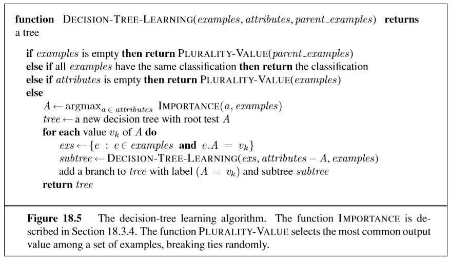
and here is the tree the algorithm learns from the examples:

generally speaking, the more examples in the training set, the better the learned tree can do in classifying new examples

Decision Trees: Splitting Using Entropy

perhaps the trickiest part of this decision tree learning algorithm is deciding what a “fairly good” choice is for a question node

one way of making this decision is to use the notion of entropy, which is an important idea from information theory

to understand the idea of entropy, suppose you have a random variable \(V\) that can be assigned one value from the set \(\{v_1, v_2, \ldots, v_k\}\)

• for simplicity we are assuming the set of possible values that \(V\) can be assigned is finite, but it is quite possible to define entropy on random variables with an infinite number of possible values

also, we assume there is a probability distribution \(P(v_k)\), which means that there is probability \(P(v_k)\) that \(V\) has the value \(v_k\)

the entropy \(H(V)\) is now defined like this:

\[\begin{split}H(V) &= \sum_{k} P(v_k) \log_2 \frac{1}{P(v_k)} \\ &= - \sum_{k} P(v_k) \log_2 P(v_k)\end{split}\]

Example. A fair coin can be modeled as a random variable \(Fair\) that has a 50% chance of being heads, and a 50% chance of being tails; its entropy \(H(Fair)\) is then calculated like this:

\[\begin{split}H(Fair) &= -(P(heads)\log_2 P(heads) + P(tails)\log_2 P(tails)) \\ &= -(\frac{1}{2}\log_2 \frac{1}{2} + \frac{1}{2}\log_2 \frac{1}{2}) \\ &= -(\log_2 \frac{1}{2}) \\ &= -(-1) \\ &= 1\end{split}\]

so \(H(Fair)=1\) for a fair coin, and we say it has 1 bit of entropy

if you re-do the calculation with an unfair coin, say a coin with a 99% chance of coming up heads, you get \(H(Unfair) \approx 0.08\) bits of entropy

in decision tree learning, if the training set has \(p\) positive examples and \(n\) negative examples, then entropy of the goal attribute of the entire set is:

\[H(Goal) = B\Big(\frac{p}{p + n}\Big)\]

here, the function \(B(q)\) is the entropy of a boolean random variable (a variable with only two possible values, true or false) and is defined like this:

\[B(q) = -(q\log_2 + (1-q)\log_2(1-q))\]

now consider some attribute \(A\) in decision tree learning; \(A\) has \(d\) different values that divides the training set of examples \(E\) into \(E_1, E_2, \ldots, E_d\)

for each of these subsets \(E_k\), suppose there are \(p_k\) positive examples and \(n_k\) negative examples; then we can define the remainder function like this:

\[\textrm{Remainder}(A) = \sum_{k=1}^{d} \frac{p_k + n_k}{p+n} B\Big(\frac{p_k}{p_k+n_k}\Big)\]

finally, the information gain of an attribute is defined like this:

\[\textrm{Gain}(A) = B\Big(\frac{p}{p+n}\Big) - \textrm{Remainder}(A)\]

the gain of an attribute \(A\) is a good way to choose how to split examples in decision tree learning: the higher the gain, the better the question

there is much more to decision tree learning, including many other algorithms and details

in practice, it is often a very good way to implement machine learning for many problems

Regression

decision trees are often a good choice for classification problems, i.e. problems where you want to learn to make a decision about, say, a yes/no question

another kind of machine learning question is prediction where your goal is to suggest the most likely numerical value for some question

for example, you could write a program that predicts the price of a house based on the square footage of the house

• intuitively, the more square footage, the higher the price
• but maybe a more precise formula can be determined

price is a number that could have many different values, and so techniques very different than decision tree learning are needed

• it’s possible you could convert this into a decision tree learning problem by replacing numeric price with classifications like “low”, “medium”, or “high”
• whether or not that change is a good idea is tough to say in general: it depends on how much detail your application needs about the price of a house

the topic of a regression has long been studied mathematics, and so we will only briefly mention it here

univariate linear regression is the simplest kind of regression, and is essentially about finding the best straight line that fits a set of training points

• of course, not all data is going to be a straight line, and so other kinds of regression would be needed for such data

in mathematical terms, the equation for a straight line on the x-y plane is \(y = w_1 x + w_2\), where \(w_1\) and \(w_2\) are usually referred to as weights

it’s convenient to define \(h_w(x) = w_1 x + w_2\), where \(w\) is the vector \([w_1, w_2]\)

given a training set of \(N\) \((x_i, y_i)\) pairs, the goal is to learn the \(h_w\) that best fits the training data; this is called linear regression

traditionally, linear regression tries to minimize this function:

\[\textrm{Loss}(h_w) = \sum_{j=1}^{N} (y_j - h_w(x_j))^2\]

that is, it minimizes the sum of the square of the differences between the known values (\(y_j\)) and value predicted by \(h_w\)

it turns out that this equation problem can be solved exactly using calculus and algebra

• that is, there an expression for \(h_w\) that gives the minimal loss — no trial and error or searching is necessary

but in general, there is usually no such closed-form solution for other regression problems, and instead gradient descent is used to find good-enough solutions

• in other words, we search for a solution that minimizes the Loss function using a variation of hill-climbing
• the exact details of how to do this for linear regression are outlined in the textbook

univariate linear regression can be generalized in a natural way to multivariate linear regression, where the space of examples are n-dimensional points (instead of being restricted to 2-dimensional points as in univariate linear regression)

• the mathematics gets a little more involved, and combines linear algebra, calculus, and programming; we won’t go into any details here

linear functions can also use be used to do classification, and perhaps the most famous example of this is the perceptron

• perceptrons were one of the early simple neural network models that were researched in the 1960s
• it turns out that perceptrons can learn only a very limited class of functions, and this caused many people to shy away from neural networks as a general approach to learning

there is much more to say about regression, but we will stop here and simply note that it is still an active area of research in statistics, mathematics, and AI

Artificial Neural Networks

neural networks have recently been very popular because they are currently the most efficient techniques for solving many useful problems image recognition and other fields

• for example, the best programs for recognizing hand-written digits learn from examples using neural networks

neural networks turn out to be an old idea: the first paper on them was in 1943 by the researchers McCulloch and Pits

• they made a simple mathematical model of a neuron that took multiple inputs and returned some output
• they showed how neural networks could represent any logical function
• but they did not know how to train such networks, i.e. how to make the networks learn functions from examples

neural nets consist of simulated neurons, often just called units, which typically have this structure:

a neural net typically consists of hundreds or thousands of such units, all connected to each other by links

• the pattern of connection varies

we say that a unit has some amount of activation, and the links between units transfer this activation

each link has a numeric weight

a unit computes a weighted sum of its input links, e.g.

\[\textrm{in}_j = \sum_{i=0}^{n}w_{i,j} a_i\]

this input value is then put through an activation function \(g\), which creates the output \(a_j\) for the unit \(j\):

\[a_j = g(\textrm{in}_j) = g\Big(\sum_{i=0}^{n}w_{i,j} a_i\Big)\]

there are a couple of common choices for the function \(g\):

• it could be a hard threshold, i.e. if \(\textrm{in}_j\) is above some fixed value tent he unit is activated; otherwise it’s not activated
• it could be a logistic function, aka sigmoid function, that looks like a little like a smooth capital S
• it could be a straight line, i.e. a sort of simple linear approximation of a logistic function

neurons can be connected together in various patterns, one of the most common being multi-layer feed forward neural nets

• typically, neurons are arranged in one or more layer, with each layer connected to the following layer only
• a hidden layer is a layer not connected to the output directly
• a single-layer neural net is a perceptron network, and it is limited in the functions it can learn
  • famously, a perceptron can’t learn the XOR (exclusive-or function)
  • perceptrons can only learn functions that are linearly separable, i.e. functions where you can draw a straight line (or hyperplane, in higher dimensions) such that all positive examples are on one side of the line, and all negative examples are on the other
• training neural nets can be done with a technique known as back propagation
  • we want to learn the weights for a neural net
  • so we can use set them in some initial way, run example input through it, and then compare the output of the network to the correct results
  • the difference between the correct results and the network can then be used to update the weights
    • see the textbook for details on the back-propagation algorithm and how it works

of course, we could say much more about neural nets: they have become a popular practical technique in many big data and learning applications

you can easily find lots of tutorials, books, courses, software libraries, etc. that will let you learn and use neural nets

k-nearest Neighbors

k-nearest neighbors (k-NN for short) is a simple learning algorithm based on the idea that the classification for a point ought to be based on the classification of points close to it

the input is a set of (x, y) points, where x are typically feature vectors, and the corresponding y is the value of the function for that x

given some new feature vector f that hasn’t been seen before, k-NN looks at the k nearest features vectors in its training set, and does the following:

• if the y values are numbers, this is a regression problem, and so f can be given a value equal to the average of its k nearest neighbors
• if the y values are members of a small class of values, this is a classification problem, and so f can be assigned a value equal to the plurality of its neighbors (i.e. the most frequent value)
  • in the case of a tie, you can conclude that f cannot be classified
  • instead of pure voting where each neighbor gets the same “power” of vote, votes might be weighted by distance, i.e. the closer a neighbor the more influence its vote has

kk-N is generally not used as a learning algorithm on its own, as other methods are faster and more accurate

but it does have some uses in particular problems, e.g. in facial recognition algorithms k-NN can be used to help with feature extraction (converting raw data in feature vectors) and dimension reduction

Unsupervised Learning

the input to an unsupervised learner is at set of examples that is not labeled with the correct output

for example, the input to an unsupervised cluster learner might be a set of (x,y) points on a graph, and its task is to find related clusters among these points

• it is not told ahead of time what the clusters are, or even how many clusters there are
• it discovers clusters on its own, and can then classify later examples as being in a particular cluster

another kind of unsupervised learner is an association rule learner

• this discovers so-called association rules among sets of items
• such a learner might be able to learn a rule like “if a set contains the x, then it probably also contains y and z”

unsupervised learning has been used in anomaly detection, e.g. for recognizing online fraud, or bringing novel patterns to the attention of a person

popular techniques for unsupervised learning include:

• k-means clustering
• certain kinds of neural nets, such as autoencoders and deep belief nets