Learned image compression (LIC) applies deep learning models to the task of image compression. It is also known as neural image compression (NIC) or deep image compression. This article introduces learned image compression, and provides a fairly brief survey of the current landscape and state-of-the-art (SOTA) context modelling approaches.
What is data compression?
The storage and transmission of data is a fundamental aspect of computing. However, every bit stored or transmitted incurs a cost. To mitigate this cost, we turn to data compression. Data compression is the process of reducing the amount of bits required to represent, store, or transmit data.
The modern age of the Internet would look very different without data compression: web pages would take much longer to load, and images and video would be much lower in resolution. The transmission of an uncompressed video stream would require thousands of times more bits than its compressed counterpart. Video streaming services such as Netflix and YouTube would suffer from a much higher operating cost, and would be much less accessible to the average consumer.
Data compression algorithms, known as codecs, are often specialized for encoding a particular type of data. Common types of data include text, images, video, audio, and point clouds. Data from such sources often contains redundancy or patterns which can be identified and eliminated by a compression algorithm to represent the data more compactly. For instance, pixels that are near each other in an image are often similar in color, which is a phenomenon known as spatial redundancy.
Data compression: an example
As an example of how data compression works, consider the random variable \( X \) representing the summer weather in the city of Vancouver, Canada. Let us say that the possible weather conditions \( (\texttt{Sunny}, \texttt{Rainy}, \texttt{Cloudy}) \) abbreviated as \( (\texttt{S}, \texttt{R}, \texttt{C}) \) are predicted to occur with the probabilities \( (\frac{1}{2}, \frac{1}{4}, \frac{1}{4}) \), respectively. To compress a sequence of weather observations \( X_1, X_2, \ldots, X_n \), we can use a codebook that maps each weather condition to a binary string: \[ \begin{align*} \texttt{S} &\rightarrow \texttt{0}, \\ \texttt{R} &\rightarrow \texttt{10}, \\ \texttt{C} &\rightarrow \texttt{11}. \end{align*} \] Then, a sequence of weather observations such as the 64-bit ASCII string “\( \texttt{SRCSSRCS} \)” can be represented more compactly as the encoded 12-bit binary string “\( \texttt{010110010110} \)”.
Notably, for any given input \( x \in \{\texttt{S}, \texttt{R}, \texttt{C}\} \), the length in bits of its encoded representation is equal to \( -\log_2 P(X = x) \). That is,
- \( -\log_2 \frac{1}{2} = 1 \text{ bit} \) for \( \texttt{S} \),
- \( -\log_2 \frac{1}{4} = 2 \text{ bits} \) for \( \texttt{R} \), and
- \( -\log_2 \frac{1}{4} = 2 \text{ bits} \) for \( \texttt{C} \).
This codebook is optimal if \( X_1, X_2, \ldots, X_n \) are independently and identically distributed (i.i.d.).
However, many raw sources studied in compression are not i.i.d. In fact, there are often patterns or correlations between consecutive elements. For instance, in the weather example, it is more likely that the weather will be \( \texttt{R} \) on a given day if it was \( \texttt{C} \) on the previous day. After a \( \texttt{C} \) is encountered, the probability distribution used for encoding should be reevaluated to a more realistic prediction, e.g. \( (\frac{1}{4}, \frac{1}{2}, \frac{1}{4}) \). The codebook must then also be updated to dynamically match this new encoding distribution: \[ \begin{align*} \texttt{S} &\rightarrow \texttt{10}, \\ \texttt{R} &\rightarrow \texttt{0}, \\ \texttt{C} &\rightarrow \texttt{11}. \end{align*} \] This is an optimal codebook for the new encoding distribution. It should be used instead of the general codebook whenever the previous weather observation is \( \texttt{C} \).
We can compress even further by determining a more accurate encoding distribution that predicts the next observation more accurately. More sophisticated probability modeling might also take into account the weather from the past several days, or from the same day in previous years. A good model might blend in other related sources of information such as past and current humidity, temperature, and wind speed. It might also analyze such information on multiple scales: locally within the city, within the province, or within the continent. Such probability modeling is the work of a meteorologist… and also a data compression researcher! In data compression, this process of determining the encoding distribution on-the-fly based on previous information is known as context modeling; and more generally, for any way of determining the encoding distribution, as entropy modeling.
Learning-based compression: the current landscape
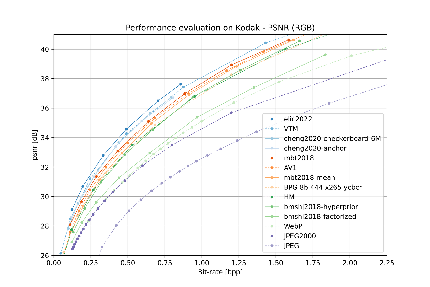
Deep learning based approaches have recently been applied to data compression. Learning-based approaches have demonstrated compression performance that is competitive with traditional standard codecs. For instance, the figure below compares the Rate-Distortion (RD) performance curves for popular and state-of-the-art (SOTA) codecs in image compression, evaluated on generic non-specialized datasets.
Learned compression has been applied to various types of data including images, video, and point clouds. For learned image compression, most prominent are approaches based on Ballé et al. 1’s compressive variational autoencoder (VAE), including 2 3 4. Other approaches based on RNNs and GANs have also been applied, including 5 6. Works in learned point cloud compression include 7 8 9 10 11, and works in learned video compression include 12 13 14 15.
Currently, one factor inhibiting industry adoption of learning-based codecs is that they are much more computationally expensive than traditional codecs like JPEG and WebP. In fact, learned compression codecs exceed reasonable computational budgets by a factor of 100–10000x. To remedy this, there is work being done towards designing low-complexity codecs for image compression, including 16 17 18 19.
Learned compression has also shown benefits when applied to learned machine or computer vision tasks. In Coding for Machines (CfM) — also referred to as Video Coding for Machines (VCM) 20 — compression is used for machine tasks such as classification, object detection, and semantic segmentation. In this paradigm, the encoder-side device compresses the input into a compact task-specialized bitstream that is transmitted to the decoder-side device or server for further inference. This idea of partially processing the input allows for significantly lower bitrates in comparison to transmitting the entire unspecialized input for inference. Extending this technique, scalable multi-task codecs such as 21 22 allocate a small base bitstream for machine tasks, and a larger enhancement bitstream for a higher-quality input reconstruction intended for human viewing.
Compression architecture overview
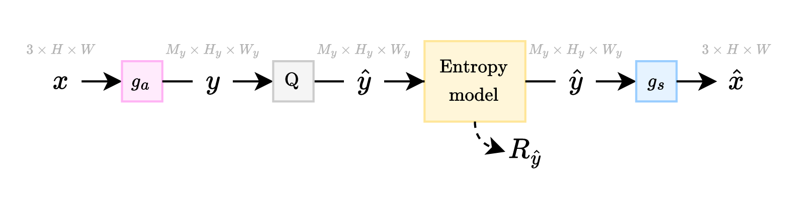
A simple compression architecture used by both traditional and learned compression methods alike is shown in Figure 2.a. In this architecture, the input \( \boldsymbol{x} \) goes through a transform \( g_a \) to generate an intermediate representation \( \boldsymbol{y} \), which is quantized to \( \boldsymbol{\hat{y}} \). Then, \( \boldsymbol{\hat{y}} \) is losslessly entropy coded to generate a transmittable bitstream from which \( \boldsymbol{\hat{y}} \) can be perfectly reconstructed at the decoder side. Finally, \( \boldsymbol{\hat{y}} \) is fed into a synthesis transform \( g_s \) which reconstructs an approximation of \( \boldsymbol{x} \), which is labeled \( \boldsymbol{\hat{x}} \). The table below lists some common choices for the components in this architecture.
| Model | Quantizer (\( \text{Q} \)) | Entropy coding | Analysis transform (\( g_a \)) | Synthesis transform (\( g_s \)) |
|---|---|---|---|---|
| JPEG | non-uniform | zigzag + RLE, Huffman | \( 8 \times 8 \) block DCT | \( 8 \times 8 \) block DCT-1 |
| JPEG 2000 | uniform dead-zone or TCQ | arithmetic | multilevel DWT | multilevel DWT-1 |
| bmshj2018-factorized | uniform | arithmetic | (Conv, GDN) \( \times 4 \) | (ConvT, IGDN) \( \times 4 \) |
Each of the components of the standard compression architecture are described in further detail below:
-
Analysis transform (\( g_a \)): The input first is transformed by the \( g_a \) transform into a transformed representation \( \boldsymbol{y} \). This transform often outputs a signal that contains less redundancy than within the input signal, and has its “energy” compacted into a smaller dimension. For instance, the JPEG codec splits the input image into \( 8 \times 8 \) blocks, then applies a discrete cosine transform (DCT) to each block. This concentrates most of the signal energy into the low-frequency components that are often the dominating frequency component within natural images. Learned compression models typically use multiple deep layers and many trainable parameters to represent the analysis transform. For instance, the bmshj2018-factorized model’s \( g_a \) transform contains 4 downsampling convolutional layers interleaved with GDN 23 nonlinear activations, totaling 1.5M to 3.5M parameters.
-
Quantization (\( \text{Q} \)): The analysis transform above outputs real numbers, i.e., \( y_i \in \mathbb{R} \). However, it is not necessary to store these values with exact precision to achieve a reasonably accurate reconstruction. Thus, we drop most of this unneeded information (e.g., \( 6.283185 \to 6 \)) by binning the values into a small discrete set of bins. Ballé et al. 1 use a uniform quantizer (i.e., “rounding”) during inference. Since this operation is non-differentiable, the quantizer is replaced with a differentiable proxy during training. For instance, Ballé et al. 1 simulate quantization error using additive unit-width uniform noise, i.e., \( \hat{y}_i = y_i + \epsilon \) where \( \epsilon \sim \mathcal{U}[-\frac{1}{2}, \frac{1}{2}] \). More recently, the straight-through estimator (STE) 24 has gained some popularity 4, where the gradients are allowed to pass through without modification, but the actual values are quantized using the same method as during inference.
-
Entropy coding: The resulting \( \boldsymbol{\hat{y}} \) is losslessly compressed using an entropy coding method. The entropy coder is targeted to match a specific encoding distribution. Whenever the encoding distribution correctly predicts an encoded symbol with high probability, the relative bit cost for encoding that symbol is reduced. Thus, some entropy models are context-adaptive, and change the encoding distribution on-the-fly in order to more accurately predict the next encoded symbol value. Recent codecs use arithmetic coding, which is particularly suited for modeling rapidly changing target encoding distributions. The CompressAI 25 implementation uses rANS 26 27, a popular recent innovation that is quite fast under certain conditions.
-
Synthesis transform (\( g_s \)): Finally, the reconstructed quantized \( \boldsymbol{\hat{y}} \) is fed into a synthesis transform \( g_s \), which produces \( \boldsymbol{\hat{x}} \). In JPEG, this is simply the inverse DCT. In learned compression, the synthesis transform consists of several deep layers and many trainable parameters. For instance, the bmshj2018-factorized model’s \( g_s \) transform contains 4 upsampling transposed convolutional layers interleaved with IGDN nonlinear activations, totaling 1.5M to 3.5M parameters.
The length of the bitstream is known as the rate cost \( R_{\boldsymbol{\hat{y}}} \), which we seek to minimize. We also seek to minimize the distortion \( D(\boldsymbol{x}, \boldsymbol{\hat{x}}) \), which is typically the mean squared error (MSE) between \( \boldsymbol{x} \) and \( \boldsymbol{\hat{x}} \). To balance these two competing goals, it is common to introduce a Lagrangian trade-off hyperparameter \( \lambda \), so that the quantity sought to be minimized is \( L = R_{\boldsymbol{\hat{y}}} + \lambda \, D(\boldsymbol{x}, \boldsymbol{\hat{x}}) \).
Entropy modeling
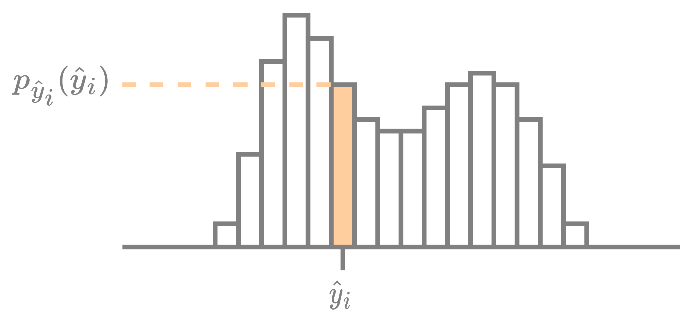
A given element \( \hat{y}_i \in \mathbb{Z} \) of the latent tensor \( \boldsymbol{\hat{y}} \) is compressed using its encoding distribution \( p_{{\hat{y}}_i} : \mathbb{Z} \to [0, 1] \), as visualized in the figure below. The rate cost for encoding \( \hat{y}_i \) is the negative log-likelihood, \( R_{{\hat{y}}_i} = -\log_2 p_{{\hat{y}}_i}({\hat{y}}_i) \), measured in bits. Afterward, the exact same encoding distribution is used by the decoder to reconstruct the encoded symbol.
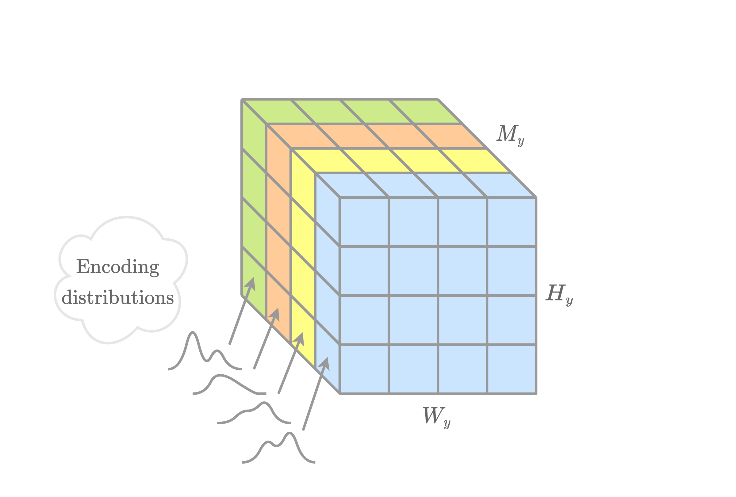
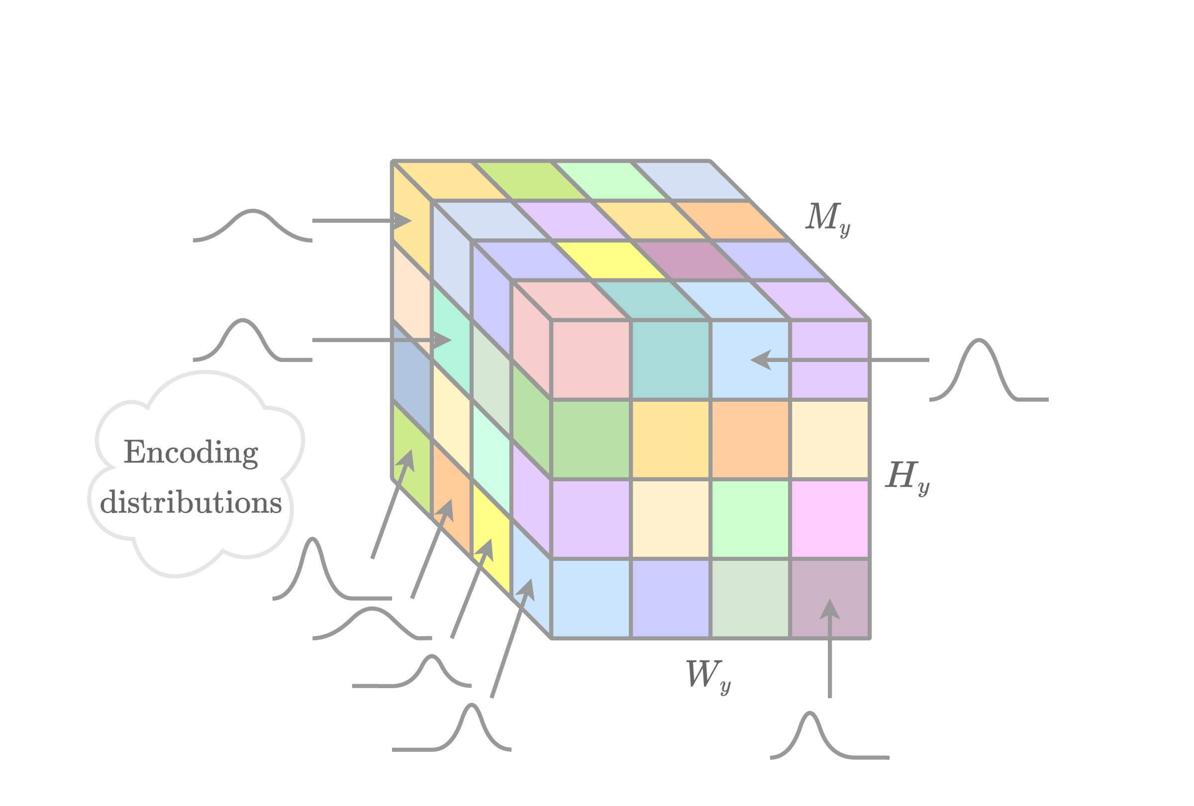
The encoding distributions are determined using an entropy model; the figure below visualizes the encoding distributions generated by well-known entropy models. These are used to compress a latent tensor \( \boldsymbol{\hat{y}} \) with dimensions \( M_y \times H_y \times W_y \). The exact total rate cost for encoding \( \boldsymbol{\hat{y}} \) using \( p_{\boldsymbol{\hat{y}}} \) is simply the sum of the negative log-likelihoods of each element, \( R_{\boldsymbol{\hat{y}}} = \sum_i -\log_2 p_{{\hat{y}}_i}({\hat{y}}_i) \).
Some popular choices for entropy models are discussed below.
Basic entropy models
“Fully factorized” entropy bottleneck
One entropy model is the “fully factorized” entropy bottleneck, as introduced by Ballé et al. 1. Let \( p_{{\hat{y}}_{c,i}} : \mathbb{Z} \to [0, 1] \) denote the probability mass distribution used to encode the \( i \)-th element \( \hat{y}_{c,i} \) from the \( c \)-th channel of \( \boldsymbol{\hat{y}} \). The same encoding distribution \( p_{{\hat{y}}_c} \) is used for all elements within the \( c \)-th channel, i.e., \( p_{{\hat{y}}_{c,i}} = p_{{\hat{y}}_c}, \forall i \). This entropy model works best when all such elements \( \hat{y}_{c,1}, \hat{y}_{c,2}, \ldots, \hat{y}_{c,N} \) are independently and identically distributed (i.i.d.).
Ballé et al. 1 model the encoding distribution as a static non-parametric distribution that is computed as the binned area under a probability density function \( f_{c} : \mathbb{R} \to \mathbb{R} \), with a corresponding cumulative distribution function \( F_{c} : \mathbb{R} \to [0, 1] \). Then, \[ \begin{equation} \label{eqn:p_y_c_integral} p_{\boldsymbol{\hat{y}}_c}(\hat{y}_{c,i}) = \int_{-\frac{1}{2}}^{\frac{1}{2}} f(\hat{y}_{c,i} + \tau) \, d\tau = F_{c}(\hat{y}_{c,i} + 1/2) - F_{c}(\hat{y}_{c,i} - 1/2). \end{equation} \] \( F_{c} \) is modelled using a small fully-connected network composed of five linear layers with channels of sizes \( [1, 3, 3, 3, 3, 1] \), whose parameters are tuned during training. Note that \( F_{c} \) is not conditioned on any other information, and is thus static.
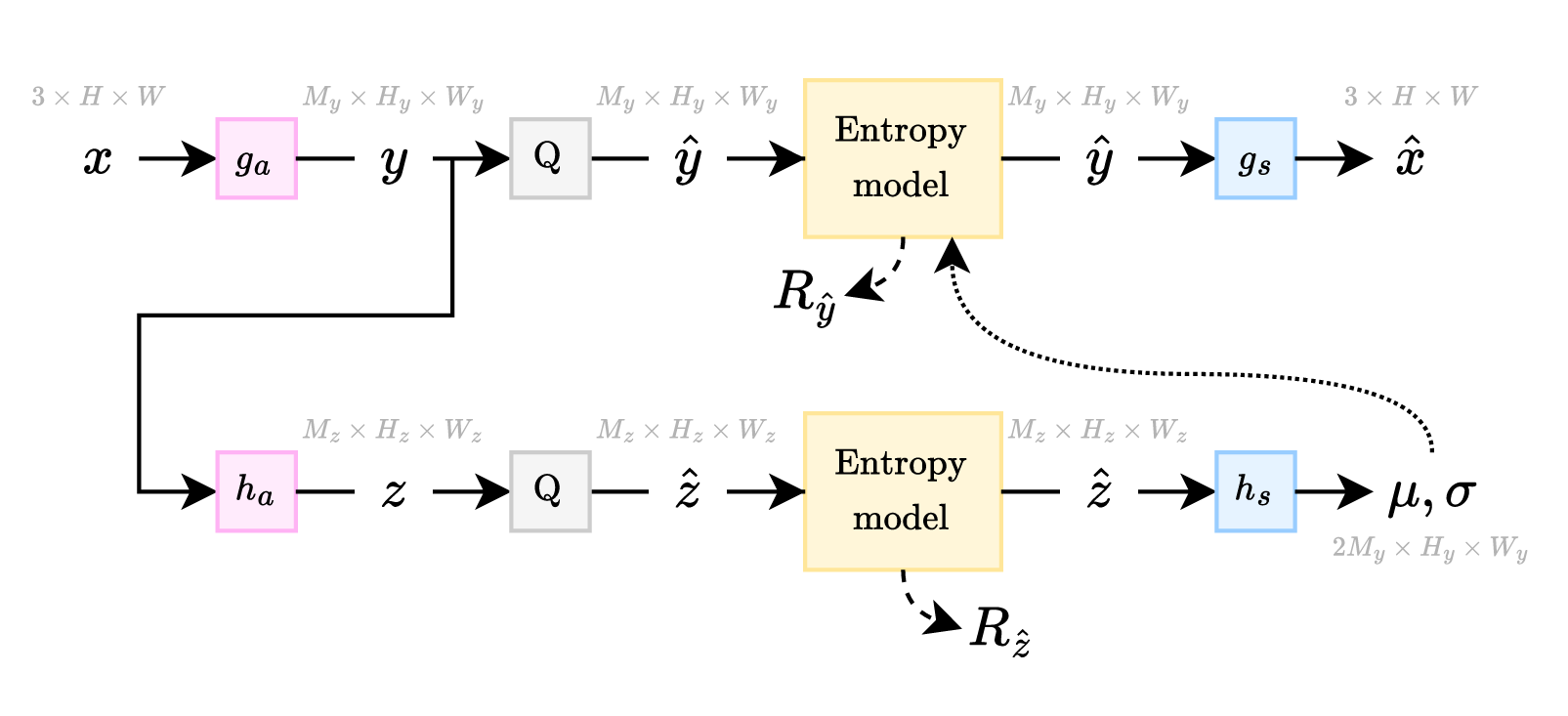
Mean-scale hyperprior
Let \( f_i(y) = \mathcal{N}(y; {\mu_i}, {\sigma_i}^2) \) be a Gaussian distribution with mean \( {\mu_i} \) and variance \( {\sigma_i}^2 \). Then, like in \( \eqref{eqn:p_y_c_integral} \), the encoding distribution \( p_{\boldsymbol{\hat{y}}_i} \) is defined as the binned area under \( f_i \): \[ \begin{equation} \label{eqn:p_y_i_integral} p_{\boldsymbol{\hat{y}}_i}(\hat{y}_i) = \int_{-\frac{1}{2}}^{\frac{1}{2}} f_i(\hat{y}_i + \tau) \, d\tau. % = F_i(\hat{y}_i + 1/2) - F_i(\hat{y}_i - 1/2). \end{equation} \] In the mean-scale variant of the “hyperprior” model introduced by Ballé et al. 1, the parameters \( {\mu_i} \) and \( {\sigma_i}^2 \) are computed by \( [{\mu_i}, {\sigma_i}] = (h_s(\boldsymbol{\hat{z}}))_i \). Here, the latent representation \( \boldsymbol{\hat{z}} = \operatorname{Quantize}[h_a(\boldsymbol{y})] \) is computed by the analysis transform \( h_a \), and then encoded using an entropy bottleneck and transmitted as side information; and \( h_s \) is a synthesis transform. This architecture is visualized in Figure 2.b. Cheng et al. 3 define \( f_i \) as a mixture of \( K \) Gaussians — known as a Gaussian mixture model (GMM) — with parameters \( {\mu}_{i}^{(k)} \) and \( {\sigma}_{i}^{(k)} \) for each Gaussian, alongside an affine combination of weights \( {w}_{i}^{(1)}, \ldots, {w}_{i}^{(K)} \) that satisfy the constraint \( \sum_k {w}_{i}^{(k)} = 1 \). A GMM encoding distribution is thus defined as \( f_i(y) = \sum_{k=1}^{K} {w}_{i}^{(k)} \, \mathcal{N}(y; {\mu}_{i}^{(k)}, [{\sigma}_{i}^{(k)}]^2) \).
Note that scale refers to the width \( \sigma_i \) of the Gaussian distribution, not to the fact that the latent \( \boldsymbol{\hat{y}} \) is spatially downsampled and then upsampled. Ballé et al. 1 originally introduced a “scale hyperprior” model, which assumes a fixed mean \( \mu_i = 0 \), though it was later shown that allowing the mean \( \mu_i \) to also vary can improve performance. In the CompressAI implementation, the scale hyperprior model constructs the encoding distributions \( p_{\boldsymbol{\hat{y}}_i} \) from the parameters \( \mu_i \) and \( \sigma_i \) using a Gaussian conditional component. The Gaussian conditional is not an entropy model on its own, by our definition. (This article defines an entropy model as a function that computes the encoding distributions \( p_{\boldsymbol{\hat{y}}} \) for a given latent tensor \( \boldsymbol{\hat{y}} \).)
Autoregressive entropy models
Let \( \boldsymbol{y} = (y_1, \ldots, y_N) \). Then, by the chain rule, the probability distribution for this sequence can be expressed as \[ \begin{equation} \label{eqn:autoregressive_full_context} p(\boldsymbol{y}) = p(y_1, \ldots, y_N) = \prod_{i=1}^{N} p(y_i | y_{1}, \ldots, y_{i-1}). \end{equation} \] This requires a fairly long context. It is common to restrict this context to a fixed number of previous elements, e.g., the previous \( K \) elements: \[ \begin{equation} p(y_i | y_{1}, \ldots, y_{i-1}) \approx p(y_i | y_{i-1}, y_{i-2}, \ldots, y_{i-K}), \end{equation} \] so that \( \eqref{eqn:autoregressive_full_context} \) becomes \[ p(\boldsymbol{y}) \approx \prod_{i=1}^{N} p(y_i | y_{i-1}, y_{i-2}, \ldots, y_{i-K}). \] An entropy model that relies upon previously decoded elements to predict the next element is known as an autoregressive context model.
Various popular choices for autoregressive context models are discussed below.
Raster scan
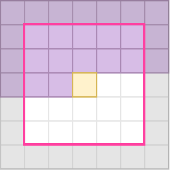
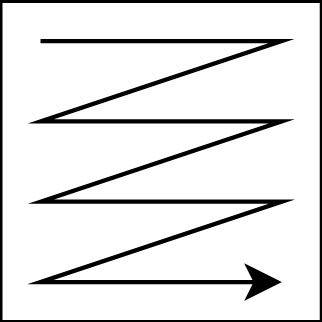
PixelCNN 28 defines an autoregressive model for 2D image data. Elements are decoded in raster-scan order, as shown in the figure below.
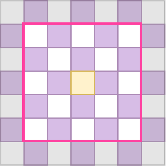
Elements that have been decoded earlier are used to help predict the encoding distribution parameters for the next element to be decoded. For the autoregressive “raster scan” decoding order, this means that all elements above the current element have been previously decoded, as have the elements to the left in the current row. In practice, only the previously decoded elements within a small neighborhood around the to-be-decoded element are considered. This is visualized in Figure 5.a.
Only the previously decoded elements should be used to predict the next element. This requirement is known as “causality”. To ensure this is accurately modelled during training, a masked convolution is applied to the quantized \( \boldsymbol{\hat{y}} \). The convolutional kernel is masked to zero out any elements that have not yet been decoded.
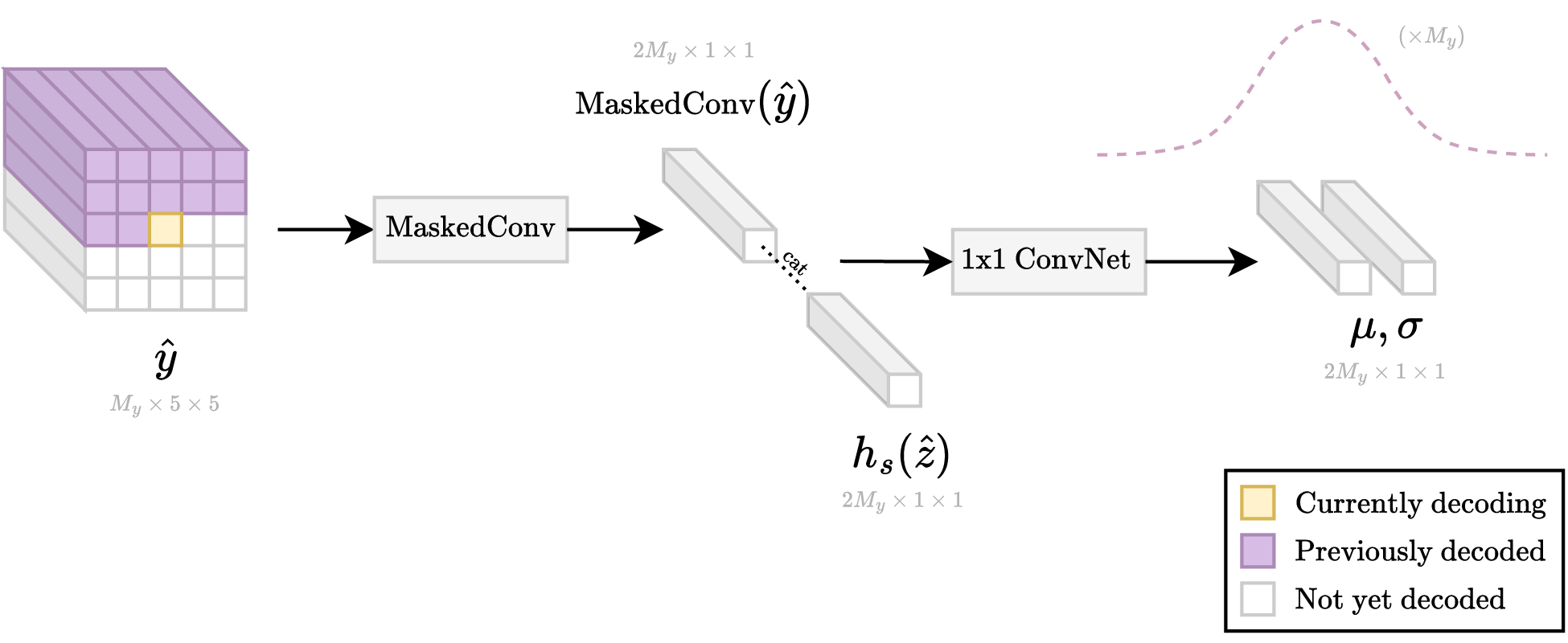
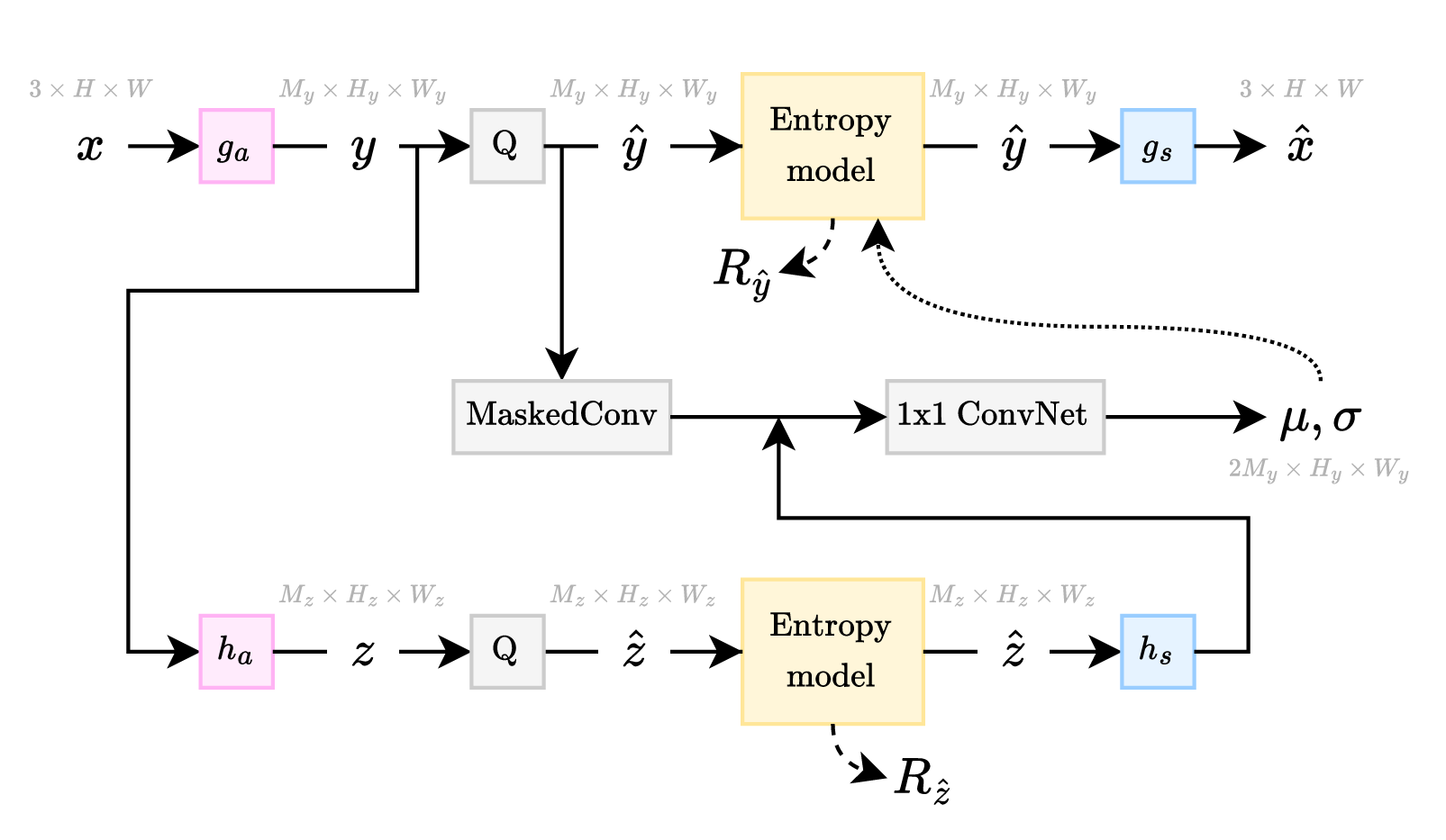
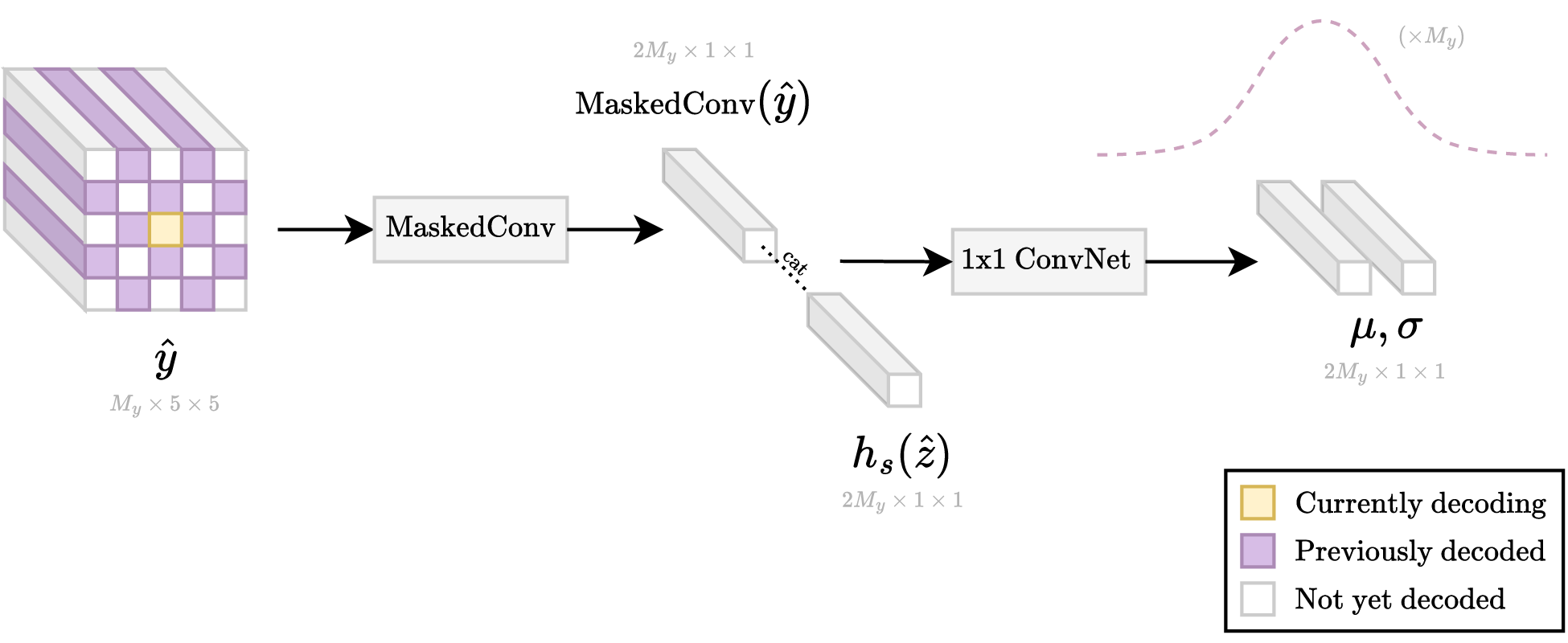
This mechanism was first used for learned image compression by Minnen et al. 2, and later by Cheng et al. 3. The high-level architecture for these autoregressive models is visualized in Figure 2.c. Figure 7 visualizes the process for decoding a \( M_y \times 1 \times 1 \) vector located at a given spatial location in the \( \boldsymbol{\hat{y}} \) latent tensor of shape \( M_y \times H_y \times W_y \). First, a masked convolution is applied to the currently decoded \( \boldsymbol{\hat{y}} \) to generate a \( 2 M_y \times 1 \times 1 \) vector. Note that all the decoded elements within the spatial window across all channels are used to generate this vector. This vector is concatenated with the corresponding colocated \( 2 M_y \times 1 \times 1 \) vector from the hyperprior side-information branch. This concatenated vector is then fed into a 1x1 ConvNet, which is a fully connected network from the perspective of the vector. This gives us the means and scales for the encoding distributions of the to-be-decoded elements within the to-be-decoded vector.
Checkerboard
Introduced by He et al. 29, the “checkerboard” context model is another autoregressive model, i.e., it uses previously decoded elements to predict the next element. In the first time step, all the even elements (known as “anchors”) are decoded. In the second time step, all the odd elements (known as “non-anchors”) are decoded. Figure 5.b visualizes the available context when decoding a non-anchor element using the previously decoded anchor elements. He et al. 29 experimentally demonstrate that the checkerboard choice of anchors is quite good since most of the predictive power comes from the immediate 4-connected neighbors.
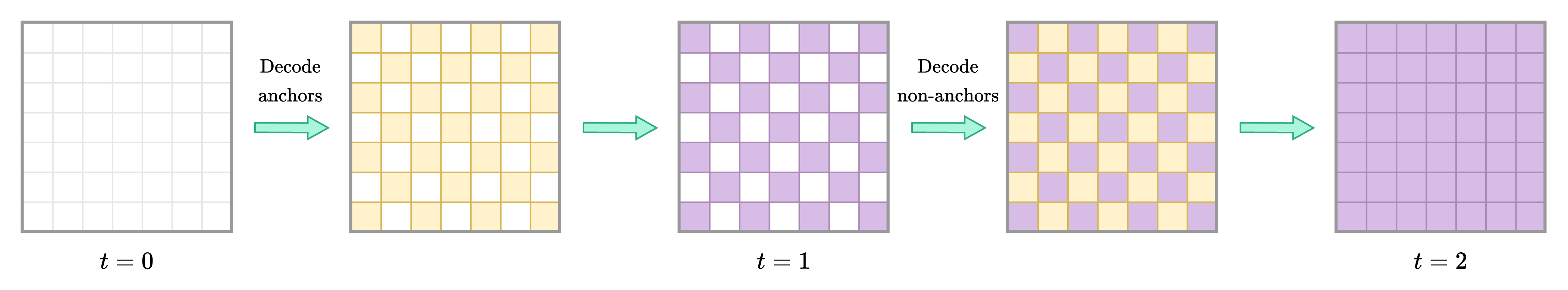
Figure 8 visualizes the latent tensor state at various time steps during the decoding process. As shown, the “checkerboard” context model only requires two time steps to decode the entire latent tensor. In contrast, the “raster scan” context model requires \( H_y \times W_y \) time steps, which increasingly grows as the image resolution increases. Thus, the “checkerboard” context model has better parallelism and is often much faster to decode. However, this comes at a cost of slightly worse RD performance compared to the “raster scan” context model. This is remedied by He et al. 4 in their “ELIC” model, which is more easily parallelizable, and exceeds the RD performance of the “raster scan” context model.
The specific process for decoding the vector for a single spatial location is visualized in Figure 9. As shown, He et al. 29 follow the exact same architectural choices as used by Minnen et al. 2 and Cheng et al. 3 for the “raster scan” context model.
Conditional channel groups
Minnen et al. 30 introduced a context model that uses previously decoded channel groups to help predict successive channel groups. He et al. 4 proposed an improvement to the original design by using unequally-sized channel groups (e.g., 16, 16, 32, 64, and 192 channels for the various groups). The order in which channel groups of different sizes are decoded is visualized in the figure below.
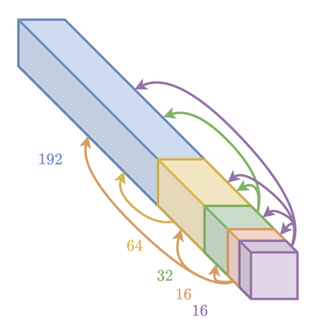
ELIC 4 uses a channel-conditional context model, which encodes each channel group using a checkerboard context model. The checkerboard context model uses information from the previously decoded channel groups alongside the hyperprior side information, as can be seen in the CompressAI implementation.
Conclusion
This article reviewed basic concepts in learned image compression, which is an ever-improving field that shows promise.
Later in this series, we will look at various popular papers, and other interesting works.
-
J. Ballé, D. Minnen, S. Singh, S. J. Hwang, and N. Johnston, “Variational image compression with a scale hyperprior,” in Proc. ICLR, 2018. Available: https://arxiv.org/abs/1802.01436 ↩︎ ↩︎ ↩︎ ↩︎ ↩︎ ↩︎ ↩︎
-
D. Minnen, J. Ballé, and G. D. Toderici, “Joint autoregressive and hierarchical priors for learned image compression,” Advances in neural information processing systems, vol. 31, 2018, Available: https://arxiv.org/abs/1809.02736 ↩︎ ↩︎ ↩︎
-
Z. Cheng, H. Sun, M. Takeuchi, and J. Katto, “Learned image compression with discretized gaussian mixture likelihoods and attention modules,” in Proc. IEEE/CVF CVPR, 2020, pp. 7939–7948. Available: https://arxiv.org/abs/2001.01568 ↩︎ ↩︎ ↩︎ ↩︎
-
D. He, Z. Yang, W. Peng, R. Ma, H. Qin, and Y. Wang, “ELIC: Efficient learned image compression with unevenly grouped space-channel contextual adaptive coding,” in Proc. IEEE/CVF CVPR, 2022, pp. 5718–5727. Available: https://arxiv.org/abs/2203.10886 ↩︎ ↩︎ ↩︎ ↩︎ ↩︎
-
G. Toderici et al., “Full resolution image compression with recurrent neural networks,” in Proc. IEEE/CVF CVPR, IEEE, 2017, pp. 5306–5314. Available: https://arxiv.org/abs/1608.05148 ↩︎
-
F. Mentzer, G. D. Toderici, M. Tschannen, and E. Agustsson, “High-fidelity generative image compression,” Advances in Neural Information Processing Systems, vol. 33, pp. 11913–11924, 2020, Available: https://proceedings.neurips.cc/paper_files/paper/2020/file/8a50bae297807da9e97722a0b3fd8f27-Paper.pdf ↩︎
-
W. Yan, Y. shao, S. Liu, T. H. Li, Z. Li, and G. Li, “Deep AutoEncoder-based lossy geometry compression for point clouds.” 2019. Available: https://arxiv.org/abs/1905.03691 ↩︎
-
Y. He, X. Ren, D. Tang, Y. Zhang, X. Xue, and Y. Fu, “Density-preserving deep point cloud compression,” in Proc. IEEE/CVF CVPR, 2022, pp. 2323–2332. Available: https://arxiv.org/abs/2204.12684 ↩︎
-
J. Pang, M. A. Lodhi, and D. Tian, “GRASP-Net: Geometric residual analysis and synthesis for point cloud compression,” in Proc. 1st int. Workshop on advances in point cloud compression, processing and analysis, 2022. Available: https://arxiv.org/abs/2209.04401 ↩︎
-
C. Fu, G. Li, R. Song, W. Gao, and S. Liu, “OctAttention: Octree-based large-scale contexts model for point cloud compression,” in Proc. AAAI, Jun. 2022, pp. 625–633. doi: 10.1609/aaai.v36i1.19942. ↩︎
-
K.-S. You, P. Gao, and Q. T. Li, “IPDAE: Improved patch-based deep autoencoder for lossy point cloud geometry compression,” in Proc. 1st int. Workshop on advances in point cloud compression, processing and analysis, 2022. Available: https://arxiv.org/abs/2208.02519 ↩︎
-
O. Rippel, S. Nair, C. Lew, S. Branson, A. G. Anderson, and L. Bourdev, “Learned video compression,” in Proc. IEEE/CVF ICCV, 2019, pp. 3454–3463. Available: https://arxiv.org/abs/1811.06981 ↩︎
-
E. Agustsson, D. Minnen, N. Johnston, J. Ballé, S. J. Hwang, and G. Toderici, “Scale-Space Flow for end-to-end optimized video compression,” in Proc. IEEE/CVF CVPR, 2020, pp. 8500–8509. Available: https://openaccess.thecvf.com/content_CVPR_2020/papers/Agustsson_Scale-Space_Flow_for_End-to-End_Optimized_Video_Compression_CVPR_2020_paper.pdf ↩︎
-
Z. Hu, G. Lu, and D. Xu, “FVC: A new framework towards deep video compression in feature space,” in Proc. IEEE/CVF CVPR, 2021, pp. 1502–1511. Available: https://arxiv.org/abs/2105.09600 ↩︎
-
Y.-H. Ho, C.-P. Chang, P.-Y. Chen, A. Gnutti, and W.-H. Peng, “CANF-VC: Conditional augmented normalizing flows for video compression,” in Proc. ECCV, Springer, 2022, pp. 207–223. Available: https://arxiv.org/abs/2207.05315 ↩︎
-
F. Galpin, M. Balcilar, F. Lefebvre, F. Racapé, and P. Hellier, “Entropy coding improvement for low-complexity compressive auto-encoders,” in Proc. IEEE DCC, 2023, pp. 338–338. Available: https://arxiv.org/abs/2303.05962 ↩︎
-
T. Ladune, P. Philippe, F. Henry, G. Clare, and T. Leguay, “COOL-CHIC: Coordinate-based low complexity hierarchical image codec,” in Proc. IEEE/CVF ICCV, 2023, pp. 13515–13522. Available: https://arxiv.org/abs/2212.05458 ↩︎
-
T. Leguay, T. Ladune, P. Philippe, G. Clare, and F. Henry, “Low-complexity overfitted neural image codec.” 2023. Available: https://arxiv.org/abs/2307.12706 ↩︎
-
F. Kamisli, “Learned lossless image compression through interpolation with low complexity,” IEEE Trans. Circuits Syst. Video Technol., pp. 1–1, 2023, Available: https://arxiv.org/abs/2212.13243 ↩︎
-
L.-Y. Duan, J. Liu, W. Yang, T. Huang, and W. Gao, “Video Coding for Machines ↩︎
-
H. Choi and I. V. Bajić, “Latent-space scalability for multi-task collaborative intelligence,” in Proc. IEEE ICIP, 2021, pp. 3562–3566. Available: https://arxiv.org/abs/2105.10089 ↩︎
-
H. Choi and I. V. Bajić, “Scalable image coding for humans and machines,” IEEE Trans. Image Process., vol. 31, pp. 2739–2754, Mar. 2022, Available: https://arxiv.org/abs/2107.08373 ↩︎
-
J. Ballé, V. Laparra, and E. P. Simoncelli, “Density modeling of images using a generalized normalization transformation,” in Proc. ICLR, 2016. Available: https://arxiv.org/abs/1511.06281 ↩︎
-
Y. Bengio, N. Léonard, and A. Courville, “Estimating or propagating gradients through stochastic neurons for conditional computation.” 2013. Available: https://arxiv.org/abs/1308.3432 ↩︎
-
J. Bégaint, F. Racapé, S. Feltman, and A. Pushparaja, “CompressAI: A PyTorch library and evaluation platform for end-to-end compression research.” 2020. Available: https://arxiv.org/abs/2011.03029 ↩︎
-
J. Duda, “Asymmetric numeral systems: Entropy coding combining speed of huffman coding with compression rate of arithmetic coding.” 2013. Available: https://arxiv.org/abs/1311.2540 ↩︎
-
F. Giesen, “Ryg_rans.” GitHub, 2014. Available: https://github.com/rygorous/ryg_rans ↩︎
-
A. van den Oord, N. Kalchbrenner, and K. Kavukcuoglu, “Pixel recurrent neural networks,” in Proc. ICML, PMLR, 2016, pp. 1747–1756. Available: https://arxiv.org/abs/1601.06759 ↩︎
-
D. He, Y. Zheng, B. Sun, Y. Wang, and H. Qin, “Checkerboard context model for efficient learned image compression,” in Proc. IEEE/CVF CVPR, 2021, pp. 14766–14775. Available: https://arxiv.org/abs/2103.15306 ↩︎ ↩︎ ↩︎
-
D. Minnen and S. Singh, “Channel-wise autoregressive entropy models for learned image compression,” in Proc. IEEE ICIP, 2020. Available: https://arxiv.org/abs/2007.08739 ↩︎