Note:
- For a detail description of the Weighted Linear Combination please refer
to Methodology.
- For a detail description of the factors/constraints used in this analysis
please refer to The
Boolean Overlay Approach
Here in the WLC, the factors are not just reclassed into 0's and 1's, but are rescaled to a particular command range according to some function. In addition, the WLC involves the production on fuzzy images in order to use fuzzy factors with the MCE module. These fuzzy factors will be standardized to a byte level range of 0- 255. However the original constraints in this project:
1) Water areas versus non water areas (WATERCON.rst) and
2) Underdeveloped land versus developed land (LANDCON.rst), will remain as Boolean images (i.e., constraining criteria) that will simply act as a mask in the last step of the WLC.
The resulting continuous factors to be produced below will be developed using fuzzy set membership functions.
The Weighted Linear Combination consists of 5 continuous factors in which have been developed by me.
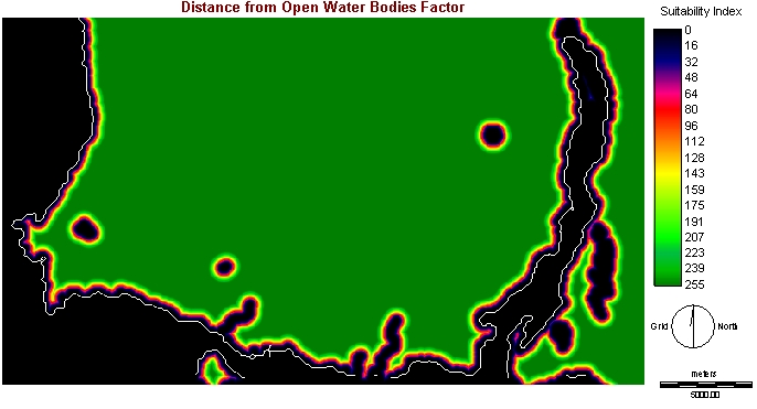
1 - Distance to Open Water Factor:
Earlier in section 4.1, I have commented that urban development to be at least 50 meters from open water bodies, and environmentalists prefer to see urban development even further from these water bodies. However, a distance of 800 meters might be just as good as a distance of 1000 meters. Suitability may not increase with distance in a constant fashion.
This involves the production of a raster image called WATERFUZZ.rst. The image was produced using the monotonically increasing Sigmoidal function to rescale the values in the distance-from-open-water bodies image (WATERDIST.rst). 100 was the value inputted for control point b and 800 was value inputted for control point for b. According to the image below, areas indicated in green show areas to be considered for urban development based on their far distances from open water bodies, while those indicated in black are not to be considered at all.
Image shown below is WATERFUZZ.rst:
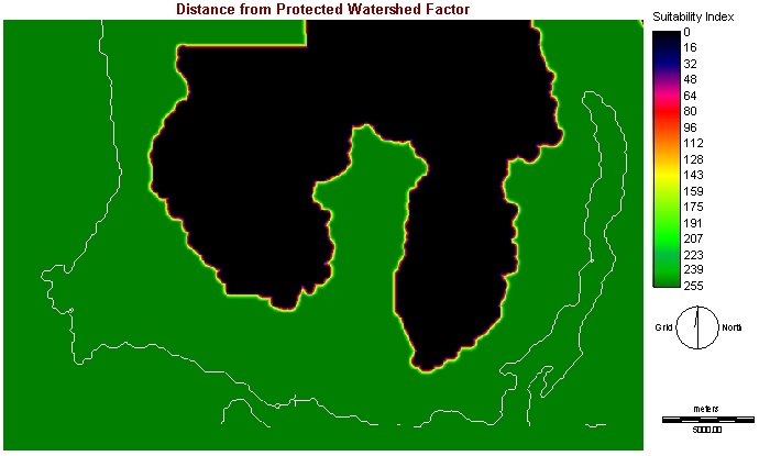
2 - Distance from Protected Watershed Factor:
Earlier in section 4.1, I have commented that urban development to be at least 100 meters from protected watersheds, and environmentalists prefer to see urban development even further from the protected watershed areas. However, a distance of 1000 meters might be just as good as a distance of 5000 meters. Suitability may not increase with distance in a constant fashion.
This involves the production of a raster image called WATERSHEDFUZZ.rst. The image was produced using the monotonically increasing Sigmoidal function to rescale the values in the distance-from-protected watersheds image (WATERSHEDDIST.rst). 100 was the value inputted for control point b and 1000 was value inputted for control point for b. According to the image below, areas indicated in green show areas to be considered for urban development based on their far distances from protected watershed areas, while those indicated in black are not to be considered at all.
Image shown below is WATERSHEDFUZZ.rst:
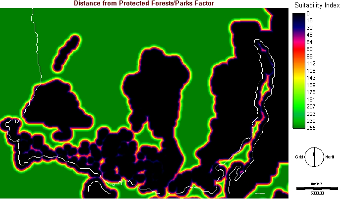
3 - Distance from Protected Park/Forest Factor:
Earlier in section 4.1, I have commented that urban development to be at least 250 meters from protected park/forest areas. However I have chosen a simple linear distance relationship for this factor because as distances from protected park/forest are increasing, the risk of forest fire spreading towards urban territory are reducing, eventually to no risk at all.
This involves the production of a raster image called FOREST_PARKFUZZ.rst. The image was produced using the monotonically increasing linear function to rescale the values in the distance-from-protected watersheds image (FOREST_PARKDIST.rst). 250 was the value inputted for control point b and 500 was value inputted for control point for b. According to the image below, areas indicated in green show areas to be considered for urban development based on their far distances from protected park/forest areas, while those indicated in black are not to be considered at all.
Image shown below is FOREST_PARKFUZZ.rst:
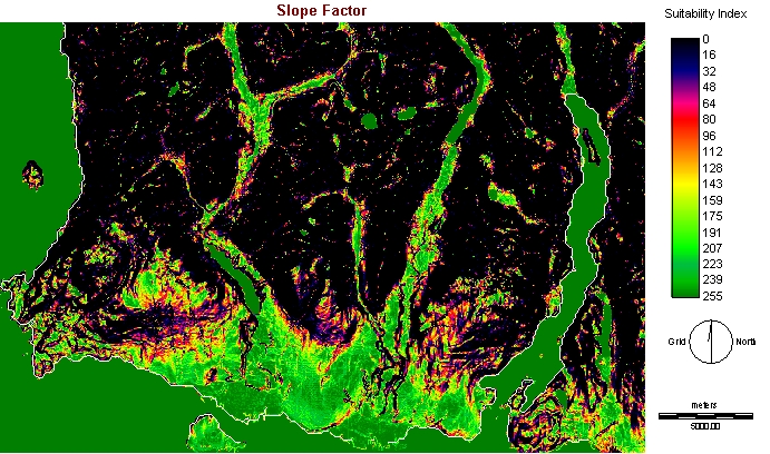
4 - Slope Factor:
From section 4.1, slopes that are not above 20% are the most cost/risk effective for development, however, the lowest slopes are the best, any slope that is above 20% is equally unsuitable.
This involves the production of a raster image called SLOPEFUZZ2.rst. The image was produced using the monotonically decreasing Sigmoidal function to rescale the values in slope image (SLOPE.rst). 0 was the value inputted for control point b and 20 was value inputted for control point for b. According to the image below, areas indicated in green show areas to be considered for urban development based on their low degree of slope, while those indicated in black are not to be considered at all.
Image shown below is SLOPEFUZZ2.rst:
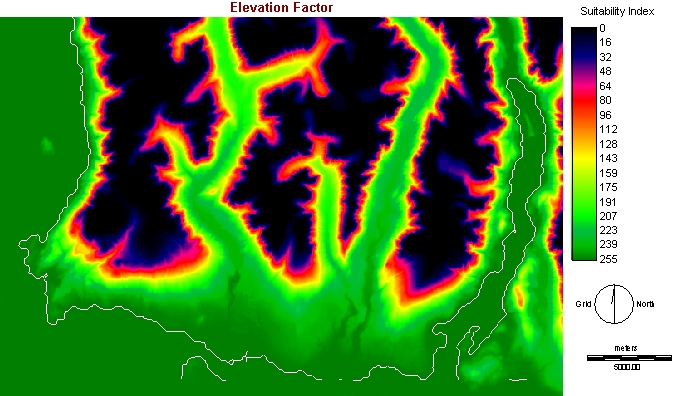
5 - Elevation Factor:
From section 4.1, areas that are not above 1000 meters are the most cost effective for development, however, the lowest areas are the best, any areas that are above 1000 meters are equally unsuitable.
This involves the production of a raster image called DEMFUZZ2.rst. The image was produced using the monotonically decreasing Sigmoidal function to rescale the values in digital elevation image (DEM_VAN.rst). 0 was the value inputted for control point b and 1000 was value inputted for control point for b. According to the image below, areas indicated in green show areas to be considered for urban development based on their low elevation levels, while those indicated in black are not to be considered at all.
Image shown below is DEM_VANFUZZ2.rst:
Note: Raster images DEM_VANFUZZ2.rst and SLOPEFUZZ2.rst have been projected to match the number of rows, columns. Min X, Max. X, Min Y, and Max. Y relative to the other fuzzy images (ex WATERFUZZ.rst). This allows the production of the final image creation of the MCE - Linear Weight Combination based upon the continuous factor 5 images of the above and the 2 constraint images discussed in section 4.1.
Please click here
for Results of the Linear Weighted Combination (4.2b)
Or click here to go back to main menu