Lecture 6
Decision Tree Learning

As discussed in the last lecture, the representation scheme we choose to represent our learned solutions and the way in which we learn those solutions are the most important aspects of a learning method. We look in this lecture at decision trees - a simple but powerful representation scheme, and we look at the ID3 method for decision tree learning.

6.1 Decision Trees

Imagine you only ever do four things at the weekend: go shopping, watch a movie, play tennis or just stay in. What you do depends on three things: the weather (windy, rainy or sunny); how much money you have (rich or poor) and whether your parents are visiting. You say to your yourself: if my parents are visiting, we'll go to the cinema. If they're not visiting and it's sunny, then I'll play tennis, but if it's windy, and I'm rich, then I'll go shopping. If they're not visiting, it's windy and I'm poor, then I will go to the cinema. If they're not visiting and it's rainy, then I'll stay in.

To remember all this, you draw a flowchart which will enable you to read off your decision. We call such diagrams decision trees. A suitable decision tree for the weekend decision choices would be as follows:

We can see why such diagrams are called trees, because, while they are admittedly upside down, they start from a root and have branches leading to leaves (the tips of the graph at the bottom). Note that the leaves are always decisions, and a particular decision might be at the end of multiple branches (for example, we could choose to go to the cinema for two different reasons).

Armed with our decision tree, on Saturday morning, when we wake up, all we need to do is check (a) the weather (b) how much money we have and (c) whether our parent's car is parked in the drive. The decision tree will then enable us to make our decision. Suppose, for example, that the parents haven't turned up and the sun is shining. Then this path through our decision tree will tell us what to do:

and hence we run off to play tennis because our decision tree told us to. Note that the decision tree covers all eventualities. That is, there are no values that the weather, the parents turning up or the money situation could take which aren't catered for in the decision tree. Note that, in this lecture, we will be looking at how to automatically generate decision trees from examples, not at how to turn thought processes into decision trees.

Reading Decision Trees

There is a link between decision tree representations and logical representations, which can be exploited to make it easier to understand (read) learned decision trees. If we think about it, every decision tree is actually a disjunction of implications (if ... then statements), and the implications are Horn clauses: a conjunction of literals implying a single literal. In the above tree, we can see this by reading from the root node to each leaf node:

If the parents are visiting, then go to the cinema
or
If the parents are not visiting and it is sunny, then play tennis
or
If the parents are not visiting and it is windy and you're rich, then go shopping
or
If the parents are not visiting and it is windy and you're poor, then go to cinema
or
If the parents are not visiting and it is rainy, then stay in.

Of course, this is just a re-statement of the original mental decision making process we described. Remember, however, that we will be programming an agent to learn decision trees from example, so this kind of situation will not occur as we will start with only example situations. It will therefore be important for us to be able to read the decision tree the agent suggests.

Decision trees don't have to be representations of decision making processes, and they can equally apply to categorisation problems. If we phrase the above question slightly differently, we can see this: instead of saying that we wish to represent a decision process for what to do on a weekend, we could ask what kind of weekend this is: is it a weekend where we play tennis, or one where we go shopping, or one where we see a film, or one where we stay in? For another example, we can refer back to the animals example from the last lecture: in that case, we wanted to categorise what class an animal was (mammal, fish, reptile, bird) using physical attributes (whether it lays eggs, number of legs, etc.). This could easily be phrased as a question of learning a decision tree to decide which category a given animal is in, e.g., if it lays eggs and is homeothermic, then it's a bird, and so on...

6.2 Learning Decision Trees Using ID3

Specifying the Problem

We now need to look at how you mentally constructed your decision tree when deciding what to do at the weekend. One way would be to use some background information as axioms and deduce what to do. For example, you might know that your parents really like going to the cinema, and that your parents are in town, so therefore (using something like Modus Ponens) you would decide to go to the cinema.

Another way in which you might have made up your mind was by generalising from previous experiences. Imagine that you remembered all the times when you had a really good weekend. A few weeks back, it was sunny and your parents were not visiting, you played tennis and it was good. A month ago, it was raining and you were penniless, but a trip to the cinema cheered you up. And so on. This information could have guided your decision making, and if this was the case, you would have used an inductive, rather than deductive, method to construct your decision tree. In reality, it's likely that humans reason to solve decisions using both inductive and deductive processes.

We can state the problem of learning decision trees as follows:

We have a set of examples correctly categorised into categories (decisions). We also have a set of attributes describing the examples, and each attribute has a finite set of values which it can possibly take. We want to use the examples to learn the structure of a decision tree which can be used to decide the category of an unseen example.

Assuming that there are no inconsistencies in the data (when two examples have exactly the same values for the attributes, but are categorised differently), it is obvious that we can always construct a decision tree to correctly decide for the training cases with 100% accuracy. All we have to do is make sure every situation is catered for down some branch of the decision tree. Of course, 100% accuracy may indicate overfitting.

The basic idea

In the decision tree above, it is significant that the "parents visiting" node came at the top of the tree. We don't know exactly the reason for this, as we didn't see the example weekends from which the tree was produced. However, it is likely that the number of weekends the parents visited was relatively high, and every weekend they did visit, there was a trip to the cinema. Suppose, for example, the parents have visited every fortnight for a year, and on each occasion the family visited the cinema. This means that there is no evidence in favour of doing anything other than watching a film when the parents visit. Given that we are learning rules from examples, this means that if the parents visit, the decision is already made. Hence we can put this at the top of the decision tree, and disregard all the examples where the parents visited when constructing the rest of the tree. Not having to worry about a set of examples will make the construction job easier.

This kind of thinking underlies the ID3 algorithm for learning decisions trees, which we will describe more formally below. However, the reasoning is a little more subtle, as (in our example) it would also take into account the examples when the parents did not visit.

Entropy

Putting together a decision tree is all a matter of choosing which attribute to test at each node in the tree. We shall define a measure called information gain which will be used to decide which attribute to test at each node. Information gain is itself calculated using a measure called entropy, which we first define for the case of a binary decision problem and then define for the general case.

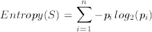
Given a binary categorisation, C, and a set of examples, S, for which the proportion of examples categorised as positive by C is p₊ and the proportion of examples categorised as negative by C is p_-, then the entropy of S is:

The reason we defined entropy first for a binary decision problem is because it is easier to get an impression of what it is trying to calculate. Tom Mitchell puts this quite well:

"In order to define information gain precisely, we begin by defining a measure commonly used in information theory, called entropy that characterizes the (im)purity of an arbitrary collection of examples."

Imagine having a set of boxes with some balls in. If all the balls were in a single box, then this would be nicely ordered, and it would be extremely easy to find a particular ball. If, however, the balls were distributed amongst the boxes, this would not be so nicely ordered, and it might take quite a while to find a particular ball. If we were going to define a measure based on this notion of purity, we would want to be able to calculate a value for each box based on the number of balls in it, then take the sum of these as the overall measure. We would want to reward two situations: nearly empty boxes (very neat), and boxes with nearly all the balls in (also very neat). This is the basis for the general entropy measure, which is defined as follows:

Given an arbitrary categorisation, C into categories c₁, ..., c_n, and a set of examples, S, for which the proportion of examples in c_i is p_i, then the entropy of S is:

This measure satisfies our criteria, because of the -p*log₂(p) construction: when p gets close to zero (i.e., the category has only a few examples in it), then the log(p) becomes a big negative number, but the p part dominates the calculation, so the entropy works out to be nearly zero. Remembering that entropy calculates the disorder in the data, this low score is good, as it reflects our desire to reward categories with few examples in. Similarly, if p gets close to 1 (i.e., the category has most of the examples in), then the log(p) part gets very close to zero, and it is this which dominates the calculation, so the overall value gets close to zero. Hence we see that both when the category is nearly - or completely - empty, or when the category nearly contains - or completely contains - all the examples, the score for the category gets close to zero, which models what we wanted it to. Note that 0*ln(0) is taken to be zero by convention.

Information Gain

We now return to the problem of trying to determine the best attribute to choose for a particular node in a tree. The following measure calculates a numerical value for a given attribute, A, with respect to a set of examples, S. Note that the values of attribute A will range over a set of possibilities which we call Values(A), and that, for a particular value from that set, v, we write S_v for the set of examples which have value v for attribute A.

The information gain of attribute A, relative to a collection of examples, S, is calculated as:

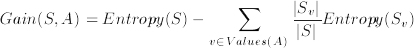
The information gain of an attribute can be seen as the expected reduction in entropy caused by knowing the value of attribute A.

An Example Calculation

As an example, suppose we are working with a set of examples, S = {s₁,s₂,s₃,s₄} categorised into a binary categorisation of positives and negatives, such that s₁ is positive and the rest are negative. Suppose further that we want to calculate the information gain of an attribute, A, and that A can take the values {v1,v2,v3}. Finally, suppose that:

s₁ takes value v2 for A
s₂ takes value v2 for A
s₃ takes value v3 for A
s₄ takes value v1 for A

To work out the information gain for A relative to S, we first need to calculate the entropy of S. To use our formula for binary categorisations, we need to know the proportion of positives in S and the proportion of negatives. These are given as: p₊ = 1/4 and p_- = 3/4. So, we can calculate:

Entropy(S) = -(1/4)log₂(1/4) -(3/4)log₂(3/4) = -(1/4)(-2) -(3/4)(-0.415) = 0.5 + 0.311 = 0.811

Note that, to do this calculation with your calculator, you may need to remember that: log₂(x) = ln(x)/ln(2), where ln(2) is the natural log of 2. Next, we need to calculate the weighted Entropy(S_v) for each value v = v1, v2, v3, v4, noting that the weighting involves multiplying by (|S_vi|/|S|). Remember also that S_v is the set of examples from S which have value v for attribute A. This means that:

S_v1 = {s₄}, s_v2={s₁, s₂}, s_v3 = {s₃}.

We now have need to carry out these calculations:

(|S_v1|/|S|) * Entropy(S_v1) = (1/4) * (-(0/1)log₂(0/1) - (1/1)log₂(1/1)) = (1/4)(-0 -(1)log₂(1)) = (1/4)(-0 -0) = 0

(|S_v2|/|S|) * Entropy(S_v2) = (2/4) * (-(1/2)log₂(1/2) - (1/2)log₂(1/2))
= (1/2) * (-(1/2)*(-1) - (1/2)*(-1)) = (1/2) * (1) = 1/2

(|S_v3|/|S|) * Entropy(S_v3) = (1/4) * (-(0/1)log₂(0/1) - (1/1)log₂(1/1)) = (1/4)(-0 -(1)log₂(1)) = (1/4)(-0 -0) = 0

Note that we have taken 0 log₂(0) to be zero, which is standard. In our calculation, we only required log₂(1) = 0 and log₂(1/2) = -1. We now have to add these three values together and take the result from our calculation for Entropy(S) to give us the final result:

Gain(S,A) = 0.811 - (0 + 1/2 + 0) = 0.311

We now look at how information gain can be used in practice in an algorithm to construct decision trees.

The ID3 algorithm

The calculation for information gain is the most difficult part of this algorithm. ID3 performs a search whereby the search states are decision trees and the operator involves adding a node to an existing tree. It uses information gain to measure the attribute to put in each node, and performs a greedy search using this measure of worth. The algorithm goes as follows:

Given a set of examples, S, categorised in categories c_i, then:

1. Choose the root node to be the attribute, A, which scores the highest for information gain relative to S.

2. For each value v that A can possibly take, draw a branch from the node.

3. For each branch from A corresponding to value v, calculate S_v. Then:

If S_v is empty, choose the category c_default which contains the most examples from S, and put this as the leaf node category which ends that branch.

If S_v contains only examples from a category c, then put c as the leaf node category which ends that branch.

Otherwise, remove A from the set of attributes which can be put into nodes. Then put a new node in the decision tree, where the new attribute being tested in the node is the one which scores highest for information gain relative to S_v (note: not relative to S). This new node starts the cycle again (from 2), with S replaced by S_v in the calculations and the tree gets built iteratively like this.

The algorithm terminates either when all the attributes have been exhausted, or the decision tree perfectly classifies the examples.

The following diagram should explain the ID3 algorithm further:

6.3 A worked example

We will stick with our weekend example. Suppose we want to train a decision tree using the following instances:

Weekend (Example) Weather Parents Money Decision (Category)

W1 Sunny Yes Rich Cinema

W2 Sunny No Rich Tennis

W3 Windy Yes Rich Cinema

W4 Rainy Yes Poor Cinema

W5 Rainy No Rich Stay in

W6 Rainy Yes Poor Cinema

W7 Windy No Poor Cinema

W8 Windy No Rich Shopping

W9 Windy Yes Rich Cinema

W10 Sunny No Rich Tennis

The first thing we need to do is work out which attribute will be put into the node at the top of our tree: either weather, parents or money. To do this, we need to calculate:

Entropy(S) = -p_cinema log₂(p_cinema) -p_tennis log₂(p_tennis) -p_shopping log₂(p_shopping) -p_{stay_in} log₂(p_{stay_in})
                   = -(6/10) * log₂(6/10) -(2/10) * log₂(2/10) -(1/10) * log₂(1/10) -(1/10) * log₂(1/10)
                   = -(6/10) * -0.737 -(2/10) * -2.322 -(1/10) * -3.322 -(1/10) * -3.322
                   = 0.4422 + 0.4644 + 0.3322 + 0.3322 = 1.571

and we need to determine the best of:

Gain(S, parents) = 1.571 - (|S_yes|/10)*Entropy(S_yes) - (|S_no|/10)*Entropy(S_no)
= 1.571 - (0.5) * 0 - (0.5) * 1.922 = 1.571 - 0.961 = 0.61

Gain(S, money) = 1.571 - (|S_rich|/10)*Entropy(S_rich) - (|S_poor|/10)*Entropy(S_poor)
= 1.571 - (0.7) * (1.842) - (0.3) * 0 = 1.571 - 1.2894 = 0.2816

This means that the first node in the decision tree will be the weather attribute. As an exercise, convince yourself why this scored (slightly) higher than the parents attribute - remember what entropy means and look at the way information gain is calculated.

From the weather node, we draw a branch for the values that weather can take: sunny, windy and rainy:

Now we look at the first branch. S_sunny = {W1, W2, W10}. This is not empty, so we do not put a default categorisation leaf node here. The categorisations of W1, W2 and W10 are Cinema, Tennis and Tennis respectively. As these are not all the same, we cannot put a categorisation leaf node here. Hence we put an attribute node here, which we will leave blank for the time being.

Looking at the second branch, S_windy = {W3, W7, W8, W9}. Again, this is not empty, and they do not all belong to the same class, so we put an attribute node here, left blank for now. The same situation happens with the third branch, hence our amended tree looks like this:

Now we have to fill in the choice of attribute A, which we know cannot be weather, because we've already removed that from the list of attributes to use. So, we need to calculate the values for Gain(S_sunny, parents) and Gain(S_sunny, money). Firstly, Entropy(S_sunny) = 0.918. Next, we set S to be S_sunny = {W1,W2,W10} (and, for this part of the branch, we will ignore all the other examples). In effect, we are interested only in this part of the table:

Weekend (Example) Weather Parents Money Decision (Category)

W1 Sunny Yes Rich Cinema

W2 Sunny No Rich Tennis

W10 Sunny No Rich Tennis

Hence we can calculate:

Gain(S_sunny, parents) = 0.918 - (|S_yes|/|S|)*Entropy(S_yes) - (|S_no|/|S|)*Entropy(S_no)
= 0.918 - (1/3)*0 - (2/3)*0 = 0.918

Gain(S_sunny, money) = 0.918 - (|S_rich|/|S|)*Entropy(S_rich) - (|S_poor|/|S|)*Entropy(S_poor)
= 0.918 - (3/3)*0.918 - (0/3)*0 = 0.918 - 0.918 = 0

Notice that Entropy(S_yes) and Entropy(S_no) were both zero, because S_yes contains examples which are all in the same category (cinema), and S_no similarly contains examples which are all in the same category (tennis). This should make it more obvious why we use information gain to choose attributes to put in nodes.

Given our calculations, attribute A should be taken as parents. The two values from parents are yes and no, and we will draw a branch from the node for each of these. Remembering that we replaced the set S by the set S_Sunny, looking at S_yes, we see that the only example of this is W1. Hence, the branch for yes stops at a categorisation leaf, with the category being Cinema. Also, S_no contains W2 and W10, but these are in the same category (Tennis). Hence the branch for no ends here at a categorisation leaf. Hence our upgraded tree looks like this:

Finishing this tree off is left as a tutorial exercise.

6.4 Avoiding Overfitting

As we discussed in the previous lecture, overfitting is a common problem in machine learning. Decision trees suffer from this, because they are trained to stop when they have perfectly classified all the training data, i.e., each branch is extended just far enough to correctly categorise the examples relevant to that branch. Many approaches to overcoming overfitting in decision trees have been attempted. As summarised by Tom Mitchell, these attempts fit into two types:

Stop growing the tree before it reaches perfection.

Allow the tree to fully grow, and then post-prune some of the branches from it.

The second approach has been found to be more successful in practice. Both approaches boil down to the question of determining the correct tree size. See Chapter 3 of Tom Mitchell's book for a more detailed description of overfitting avoidance in decision tree learning.

6.5 Appropriate Problems for Decision Tree Learning

It is a skilled job in AI to choose exactly the right learning representation/method for a particular learning task. As elaborated by Tom Mitchell, decision tree learning is best suited to problems with these characteristics:

The background concepts describe the examples in terms of attribute-value pairs, and the values for each attribute range over finitely many fixed possibilities.

The concept to be learned (Mitchell calls it the target function) has discrete values.

Disjunctive descriptions might be required in the answer.