Polynomial Distributed Lag Estimation

The PDLREG Procedure

Polynomial Distributed Lag Estimation

The simple finite distributed lag model is expressed in the form

$y_{t} = {\alpha} + \sum_{i=0}^p{{\beta}_{i}x_{t-i}} + {\epsilon}_{t}$

When the lag length (p) is long, severe multicollinearity can occur. Use the Almon or polynomial distributed lag model to avoid this problem, since the relatively low degree d ( ${{\le} p}$ ) polynomials can capture the true lag distribution. The lag coefficient can be written in the Almon polynomial lag

${\beta}_{i} = {\alpha}_{0}^{*} + \sum_{j=1}^d{{\alpha}_{j}^{*} i^j}$

Emerson (1968) proposed an efficient method of constructing orthogonal polynomials from the preceding polynomial equation as

${\beta}_{i} = {\alpha}_{0} + \sum_{j=1}^d{{\alpha}_{j} f_{j}(i)}$

where f_j(i) is a polynomial of degree j in the lag length i. The polynomials f_j(i) are chosen so that they are orthogonal:

$\sum_{i=1}^n{w_{i}f_{j}(i)f_{k}(i)} = \cases{ 1 & \hspace*{1em}\rm{if} j = k\space \cr 0 & \hspace*{1em}\rm{if} j {\neq} k\space }$

where w_i is the weighting factor, and n = p+1 . PROC PDLREG uses the equal weights (w_i = 1) for all i. To construct the orthogonal polynomials, the following recursive relation is used:

f_j(i) = (A_ji + B_j)f_j-1(i) - C_jf_j-2(i) j = 1, ... , d

The constants A_j, B_j, and C_j are determined as follows:

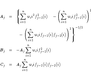
$A_{j} &=& \{ \sum_{i=1}^n{w_{i}i^2f_{j-1}^2(i)} \hspace*{1em}-(\sum_{i=1}^n{w_{... ...{w_{i}i f_{j-1}^2(i)} \ C_{j} &=& A_{j}\sum_{i=1}^n{w_{i}i f_{j-1}(i)f_{j-2}(i)}$

where f_-1(i)=0 and ${f_{0}(i)=1/\sqrt{\sum_{i=1}^n{w_{i}}} }$ .

PROC PDLREG estimates the orthogonal polynomial coefficients, ${{\alpha}_{0},{ ... },{\alpha}_{d}}$ ,to compute the coefficient estimate of each independent variable (X) with distributed lags. For example, if an independent variable is specified as X(9,3), a third-degree polynomial is used to specify the distributed lag coefficients. The third-degree polynomial is fit as a constant term, a linear term, a quadratic term, and a cubic term. The four terms are constructed to be orthogonal. In the output produced by the PDLREG procedure for this case, parameter estimates with names X**0, X**1, X**2, and X**3 correspond to ${\hat{{\alpha}}_{0}, \hat{{\alpha}}_{1}, \hat{{\alpha}}_{2}}$ , and ${\hat{{\alpha}}_{3}}$ , respectively. A test using the t statistic and the approximate p-value ("Approx Pr > |t|") associated with X**3 can determine whether a second-degree polynomial rather than a third-degree polynomial is appropriate. The estimates of the ten lag coefficients associated with the specification X(9,3) are labeled X(0), X(1), X(2), X(3), X(4), X(5), X(6), X(7), X(8), and X(9).

Chapter Contents
Previous
Next
Top