Relation of ARMA and State Space Forms

The STATESPACE Procedure

Relation of ARMA and State Space Forms

Every state space model has an ARMA representation, and conversely every ARMA model has a state space representation. This section discusses this equivalence. The following material is adapted from Akaike (1974), where there is a more complete discussion. Pham-Dinh-Tuan (1978) also contains a discussion of this material.

Suppose you are given the following ARMA model:

${\Phi}(B)x_{t}={\Theta}(B)e_{t}$

or, in more detail

$x_{t}-{\Phi}_{1}x_{t-1}- { ... }-{\Phi}_{p}x_{t-p} = e_{t}+{\Theta}_{1}e_{t-1}+ { ... }+{\Theta}_{q}e_{t-q}$ (1)

where e_t is a sequence of independent multivariate normal random vectors with mean 0 and variance matrix ${{\Sigma}_{ee}}$ ;B is the backshift operator (Bx_t = x_t-1); ${{\Phi}(B)}$ and ${{\Theta}(B)}$ are matrix polynomials in B; and x_t is the observed process.

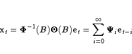
If the roots of the determinantial equation ${{|{\Phi}(B)|} = 0}$ are outside the unit circle in the complex plane, the model can also be written as

$x_{t} = {\Phi}^{-1}(B){\Theta}(B)e_{t} = \sum_{i=0}^{{\infty}}{{\Psi}_{i}e_{t-i} }$

The ${{\Psi}_{i}}$ matrices are known as the impulse response matrices and can be computed as ${{\Phi}^{-1}(B){\Theta}(B)}$ . You can assume p>q since, if this is not initially true, you can add more terms ${{\Phi}_{i}}$ that are identically 0 without changing the model.

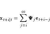
To write this set of equations in a state space form, proceed as follows. Let ${x_{t+i| t}}$ be the conditional expectation of x_t+i given x_w for ${w {\leq} t}$ .The following relations hold:

$x_{t+i| t} = \sum_{j=i}^{{\infty}}{{\Psi}_{j}e_{t+i-j} }$

$x_{t+i| t+1} = x_{t+i| t}+{\Psi}_{i-1}e_{t+1}$

However, from equation (1) you can derive the following relationship:

$x_{t+p| t} = {\Phi}_{1}x_{t+p-1| t}+{ ... }+{\Phi}_{p}x_{t}$ (2)

Hence, when i=p, you can substitute for ${x_{t+p| t}}$ in the right-hand side of equation (2) and close the system of equations.

This substitution results in the following model in the state space form z_t+1 = Fz_t+Ge_t+1:

$[\matrix{ x_{t+1} \cr x_{t+2| t+1} \cr {\vdots} \cr x_{t+p| t+1} } ] = [\matr... ...] + [\matrix{ I \cr {\Psi}_{1} \cr {\vdots} \cr {\Psi}_{p-1} \cr } ] e_{t+1}$

Note that the state vector z_t is composed of conditional expectations of x_t and the first r components of z_t are equal to x_t.

The state space form can be cast into an ARMA form by solving the system of difference equations for the first r components.

When converting from an ARMA form to a state space form, you can generate a state vector larger than needed; that is, the state space model may not be a minimal representation. When going from a state space form to an ARMA form, you can have nontrivial common factors in the autoregressive and moving average operators that yield an ARMA model larger than necessary.

If the state space form used is not a minimal representation, some but not all components of ${x_{t+i| t}}$ may be linearly dependent. This situation corresponds to ${[{\Phi}_{p} {\Theta}_{p-1} ] }$ being of less than full rank when ${{\Phi}(B)}$ and ${{\Theta}(B)}$ have no common nontrivial left factors. In this case, z_t consists of a subset of the possible components of ${[x_{t+i| t}] i=1, 2,{ ... }, p-1. }$ However, once a component of ${x_{t+i| t}}$ (for example, the jth one) is linearly dependent on the previous conditional expectations, then all subsequent jth components of ${x_{t+k| t}}$ for k > i must also be linearly dependent. Note that in this case, equivalent but seemingly different structures can arise if the order of the components within x_t is changed.

Chapter Contents
Previous
Next
Top