Computational Details

Chapter Contents

The SYSLIN Procedure

Computational Details

This section discusses various computational details.

Computation of Model Crossproduct Matrix

Model crossproduct matrix X'X is formed from projected values. For K-class estimation,

X = (1-k) R + k Z(Z'Z)^-1Z' R

where Z is the instrument set and R is the the regressor set. Note that k=1 for the 2SLS method and k=0 for the OLS method.

In the 3SLS, IT3SLS, SUR, and ITSUR methods, X'X is formed as

$X'X = R' (S^{-1} \otimes Z(Z'Z)^{-1}Z') R$

where Z and R are as defined previously and S is an estimate of the cross-equation covariance matrix. For SUR and ITSUR, Z is the identity matrix.

Computation of Standard Errors

The VARDEF= option in the PROC SYSLIN statement controls the denominator used in calculating the cross-equation covariance estimates and the parameter standard errors and covariances. The values of the VARDEF= option and the resulting denominator are as follows:

N: uses the number of nonmissing observations.
DF: uses the number of nonmissing observations less the degrees of freedom in the model.
WEIGHT: uses the sum of the observation weights given by the WEIGHTS statement.
WDF: uses the sum of the observation weights given by the WEIGHTS statement less the degrees of freedom in the model.

The VARDEF= option does not affect the model mean square error, root mean square error, or R² statistics. These statistics are always based on the error degrees of freedom, regardless of the VARDEF= option. The VARDEF= option also does not affect the dependent variable coefficient of variation (C.V.).

Reduced Form Estimates

The REDUCED option on the PROC SYSLIN statement computes estimates of the reduced form coefficients. The REDUCED option requires that the equation system be square. If there are fewer models than endogenous variables, IDENTITY statements can be used to complete the equation system.

The reduced form coefficients are computed as follows. Represent the equation system, with all endogenous variables moved to the left-hand side of the equations and identities, as:

${B Y} = {{\Gamma} X}$

Here B is the estimated coefficient matrix for the endogenous variables Y, and ${\Gamma}$ is the estimated coefficient matrix for the exogenous (or predetermined) variables X.

The system can be solved for Y as follows, provided B is square and nonsingular:

$Y = B^{-1} {{\Gamma} X}$

The reduced form coefficients are the matrix ${ B^{-1} {{\Gamma}}}$ .

Uncorrelated Errors Across Equations

The SDIAG option in the PROC SYSLIN statement computes estimates assuming uncorrelated errors across equations. As a result, when the SDIAG option is used, the 3SLS estimates are identical to 2SLS estimates, and the SUR estimates are the same as the OLS estimates.

Over Identification Restrictions

The OVERID option in the MODEL statement can be used to test for over identifying restrictions on parameters of each equation. The null hypothesis is that the predetermined variables not appearing in any equation have zero coefficients. The alternative hypothesis is that at least one of the assumed zero coefficients is nonzero. The test is approximate and rejects the null hypothesis too frequently for small sample sizes.

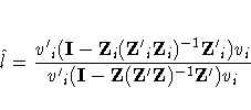
The formula for the test is given as follows. Let ${y_{i} = {\beta}_{i}Y_{i} + {\gamma}_{i}Z_{i} + e_{i}}$ be the ith equation. Y_i are the endogenous variables that appear as regressors in the ith equation, and Z_i are the instrumental variables that appear as regressors in the ith equation. Let N_i be the number of variables in Y_i and Z_i.

Let ${v_{i} = y_{i}-Y_{i}\hat{{\beta}_{i}}}$ . Let Z represent all instrumental variables, T be the total number of observations, and K be the total number of instrumental variables. Define ${\hat{l}}$ as follows:

$\hat{l} = \frac{{v'}_{i}(I-Z_{i}({Z'}_{i}Z_{i})^{-1}{Z'}_{i})v_{i}}{{v'}_{i}(I-Z({Z'}Z)^{-1}{Z'})v_{i} }$

Then the test statistic

$\frac{T-K}{K-N_{i} } ( \hat{l} - 1 )$

is distributed approximately as an F with K-N_i and T-K degrees of freedom. Refer to Basmann (1960) for more information.

Fuller's Modification to LIML

The ALPHA= option in the PROC SYSLIN and MODEL statements parameterizes Fuller's modification to LIML. This modification is ${k={\gamma}-({\alpha}/(n-g))}$ , where ${\alpha}$ is the value of the ALPHA= option, ${\gamma}$ is the LIML k value, n is the number of observations, and g is the number of predetermined variables. Fuller's modification is not used unless the ALPHA= option is specified. Refer to Fuller (1977) for more information.

Chapter Contents
Previous
Next
Top