Basic Seasonal Adjustment
Suppose you have monthly retail sales data
starting in September, 1978, in a SAS
data set named SALES. At this point you do not suspect
that any calendar effects are present and there are no
prior adjustments that need to be made to the data.
In this simplest case, you need only specify the DATE=
variable in the MONTHLY statement, which associates a
SAS date value to each observation. To see the results
of the seasonal adjustment, you must request table D11, the final
seasonally adjusted series, in a TABLES statement.
   data sales;
      input sales @@;
      date = intnx( 'month', '01sep1978'd, _n_-1 );
      format date monyy7.;
      datalines;
   run;

   proc x11 data=sales;
      monthly date=date;
      var sales;
      tables d11;
   run;
|
| X-11 Seasonal Adjustment Program |
| U. S. Bureau of the Census |
| Economic Research and Analysis Division |
| November 1, 1968 |
| |
| The X-11 program is divided into seven major parts. |
| Part Description |
| A. Prior adjustments, if any |
| B. Preliminary estimates of irregular component weights |
| and regression trading day factors |
| C. Final estimates of above |
| D. Final estimates of seasonal, trend-cycle and |
| irregular components |
| E. Analytical tables |
| F. Summary measures |
| G. Charts |
| |
| Series - sales |
| Period covered - 9/1978 to 8/1990 |
| Type of run: multiplicative seasonal adjustment. |
| No printout. No charts. |
| Sigma limits for graduating extreme values are 1.5 and 2.5 |
| Irregular values outside of 2.5-sigma limits are excluded |
| from trading day regression |
|
| The X11 Procedure |
| Seasonal Adjustment of - sales |
| D11 Final Seasonally Adjusted Series |
| Year |
JAN |
FEB |
MAR |
APR |
MAY |
JUN |
JUL |
AUG |
SEP |
OCT |
NOV |
DEC |
Total |
| 1978 |
. |
. |
. |
. |
. |
. |
. |
. |
123.507 |
125.776 |
124.735 |
129.870 |
503.887 |
| 1979 |
124.935 |
126.533 |
125.282 |
125.650 |
127.754 |
129.648 |
127.880 |
129.285 |
126.562 |
134.905 |
133.356 |
136.117 |
1547.91 |
| 1980 |
128.734 |
139.542 |
143.726 |
143.854 |
148.723 |
144.530 |
140.120 |
153.475 |
159.281 |
162.128 |
168.848 |
165.159 |
1798.12 |
| 1981 |
176.329 |
166.264 |
167.433 |
167.509 |
173.573 |
175.541 |
179.301 |
182.254 |
187.448 |
197.431 |
184.341 |
184.304 |
2141.73 |
| 1982 |
186.747 |
202.467 |
192.024 |
202.761 |
197.548 |
206.344 |
211.690 |
213.691 |
214.204 |
218.060 |
228.035 |
240.347 |
2513.92 |
| 1983 |
233.109 |
223.345 |
218.179 |
226.389 |
224.249 |
227.700 |
222.045 |
222.127 |
222.835 |
212.227 |
230.187 |
232.827 |
2695.22 |
| 1984 |
238.261 |
239.698 |
246.958 |
242.349 |
244.665 |
247.005 |
251.247 |
253.805 |
264.924 |
266.004 |
265.366 |
277.025 |
3037.31 |
| 1985 |
275.766 |
282.316 |
294.169 |
285.034 |
294.034 |
296.114 |
294.196 |
309.162 |
311.539 |
319.518 |
318.564 |
323.921 |
3604.33 |
| 1986 |
325.471 |
332.228 |
330.401 |
330.282 |
333.792 |
331.349 |
337.095 |
341.127 |
346.173 |
350.183 |
360.792 |
362.333 |
4081.23 |
| 1987 |
363.592 |
373.118 |
368.670 |
377.650 |
380.316 |
376.297 |
379.668 |
375.607 |
374.257 |
372.672 |
368.135 |
364.150 |
4474.13 |
| 1988 |
370.966 |
384.743 |
386.833 |
405.209 |
380.840 |
389.132 |
385.479 |
377.147 |
397.404 |
403.156 |
413.843 |
416.142 |
4710.89 |
| 1989 |
428.276 |
418.236 |
429.409 |
446.467 |
437.639 |
440.832 |
450.103 |
454.176 |
460.601 |
462.029 |
427.499 |
485.113 |
5340.38 |
| 1990 |
480.631 |
474.669 |
486.137 |
483.140 |
481.111 |
499.169 |
485.370 |
485.103 |
. |
. |
. |
. |
3875.33 |
| Avg |
277.735 |
280.263 |
282.435 |
286.358 |
285.354 |
288.638 |
288.683 |
291.413 |
265.728 |
268.674 |
268.642 |
276.442 |
|
| Total: 40324 Mean: 280.03 S.D.: 111.31 |
|
Figure 21.1: Basic Seasonal Adjustment
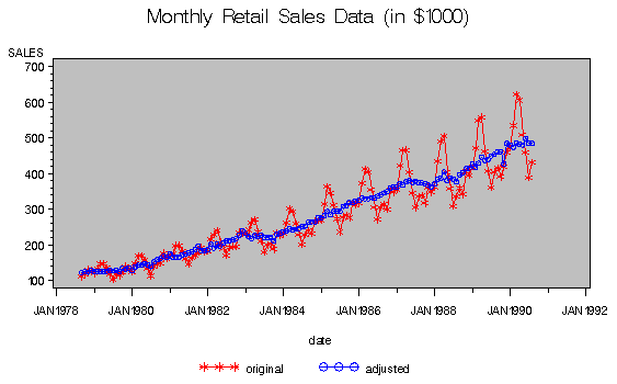
You can compare the original series, table B1, and
the final seasonally adjusted series, table D11 by
plotting them together. These tables are requested
and named in the OUTPUT statement.
   title 'Monthly Retail Sales Data (in $1000)';

   proc x11 data=sales noprint;
      monthly date=date;
      var sales;
      output out=out b1=sales d11=adjusted;
   run;

   symbol1 i=join v='star';
   symbol2 i=join v='circle';
   legend1 label=none value=('original' 'adjusted');

   proc gplot data=out;
      plot sales    * date = 1
           adjusted * date = 2 / overlay legend=legend1;
   run;
Figure 21.2: Plot of Original and Seasonally Adjusted Data
Copyright © 1999 by SAS Institute Inc., Cary, NC, USA. All rights reserved.