Equations for the Smoothing Models

Chapter Contents

Forecasting Process Details

Equations for the Smoothing Models

Simple Exponential Smoothing

The model equation for simple exponential smoothing is

$Y_{t} = {\mu}_{t} + {\epsilon}_{t}$

The smoothing equation is

$L_{t} = {\alpha}Y_{t} + (1-{\alpha})L_{t-1}$

The error-correction form of the smoothing equation is

$L_{t} = L_{t-1} + {\alpha}e_{t}$

(Note: For missing values, e_t=0.)

The k-step prediction equation is

$\hat{Y}_{t}(k) = L_{t}$

The ARIMA model equivalency to simple exponential smoothing is the ARIMA(0,1,1) model

$(1-B)Y_{t} = (1-{\theta}B){\epsilon}_{t}$

${\theta} = 1 - {\alpha}$

The moving-average form of the equation is

$Y_{t} = {\epsilon}_{t} + \sum_{j=1}^{{\infty}}{{\alpha}{\epsilon}_{t-j}}$

For simple exponential smoothing, the additive-invertible region is

$\{ 0 \lt {\alpha} \lt 2\}$

The variance of the prediction errors is estimated as

${var}(e_{t}(k)) = {var}({\epsilon}_{t}) [{\ssbeleven 1 + \sum_{j=1}^{k-1}{{\alpha}^2}}] = {var}({\epsilon}_{t})( 1 + (k-1){\alpha}^2)$

Double (Brown) Exponential Smoothing

The model equation for double exponential smoothing is

$Y_{t} = {\mu}_{t} + {\beta}_{t}t + {\epsilon}_{t}$

The smoothing equations are

$L_{t} = {\alpha}Y_{t} + (1-{\alpha})L_{t-1}$

$T_{t} = {\alpha}(L_{t} - L_{t-1}) + (1-{\alpha})T_{t-1}$

This method may be equivalently described in terms of two successive applications of simple exponential smoothing:

$S_{t}^{{\ssbeleven [1]}} = {\alpha}Y_{t} + (1-{\alpha}) S_{t-1}^{{\ssbeleven [1]}}$

$S_{t}^{{\ssbeleven [2]}} = {\alpha} S_{t}^{{\ssbeleven [1]}} + (1-{\alpha}) S_{t-1}^{{\ssbeleven [2]}}$

where S_t^[1] are the smoothed values of Y_t and S_t^[2] are the smoothed values of S_t^[1]. The prediction equation then takes the form:

$\hat{Y}_{t}(k) = (2+{\alpha}k/(1-{\alpha})) S_{t}^{{\ssbeleven [1]}} - (1+{\alpha}k/(1-{\alpha})) S_{t}^{{\ssbeleven [2]}}$

The error-correction form of the smoothing equations is

$L_{t} = L_{t-1} + T_{t-1} + {\alpha}e_{t}$

$T_{t} = T_{t-1} + {\alpha}^2e_{t}$

(Note: For missing values, e_t=0.)

The k-step prediction equation is

$\hat{Y}_{t}(k) = L_{t} + ( (k-1) + 1/{\alpha} )T_{t}$

The ARIMA model equivalency to double exponential smoothing is the ARIMA(0,2,2) model

$(1-B)^2Y_{t} = (1-{\theta}B)^2{\epsilon}_{t}$

${\theta} = 1 - {\alpha}$

The moving-average form of the equation is

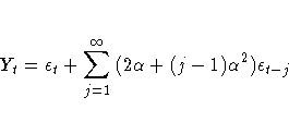
$Y_{t} = {\epsilon}_{t} + \sum_{j=1}^{{\infty}}{(2{\alpha} + (j-1){\alpha}^2) {\epsilon}_{t-j}}$

For double exponential smoothing, the additive-invertible region is

$\{ 0 \lt {\alpha} \lt 2\}$

The variance of the prediction errors is estimated as

${var}(e_{t}(k)) = {var}({\epsilon}_{t}) [{\ssbeleven 1 + \sum_{j=1}^{k-1}{(2{\alpha} + (j-1){\alpha}^2)^2}}]$

Linear (Holt) Exponential Smoothing

The model equation for linear exponential smoothing is

$Y_{t} = {\mu}_{t} + {\beta}_{t}t + {\epsilon}_{t}$

The smoothing equations are

$L_{t} = {\alpha}Y_{t} + (1-{\alpha})(L_{t-1} + T_{t-1})$

$T_{t} = {\gamma}(L_{t} - L_{t-1}) + (1-{\gamma})T_{t-1}$

The error-correction form of the smoothing equations is

$L_{t} = L_{t-1} + T_{t-1} + {\alpha}e_{t}$

$T_{t} = T_{t-1} + {\alpha}{\gamma}e_{t}$

(Note: For missing values, e_t=0.)

The k-step prediction equation is

$\hat{Y}_{t}(k) = L_{t} + kT_{t}$

The ARIMA model equivalency to linear exponential smoothing is the ARIMA(0,2,2) model

$(1-B)^2Y_{t} = (1-{\theta}_{1}B-{\theta}_{2}B^2) {\epsilon}_{t}$

${\theta}_{1} = 2 - {\alpha} - {\alpha}{\gamma}$

${\theta}_{2} = {\alpha} - 1$

The moving-average form of the equation is

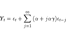
$Y_{t} = {\epsilon}_{t} + \sum_{j=1}^{{\infty}}{({\alpha} + j{\alpha}{\gamma}) {\epsilon}_{t-j}}$

For linear exponential smoothing, the additive-invertible region is

$\{ 0 \lt {\alpha} \lt 2\}$

$\{ 0 \lt {\gamma} \lt 4/{\alpha} - 2\}$

The variance of the prediction errors is estimated as

${var}(e_{t}(k)) = {var}({\epsilon}_{t}) [{\ssbeleven 1 + \sum_{j=1}^{k-1}{({\alpha} + j{\alpha}{\gamma})^2}}]$

Damped-Trend Linear Exponential Smoothing

The model equation for damped-trend linear exponential smoothing is

$Y_{t} = {\mu}_{t} + {\beta}_{t}t + {\epsilon}_{t}$

The smoothing equations are

$L_{t} = {\alpha}Y_{t} + (1-{\alpha})(L_{t-1} + {\phi}T_{t-1})$

$T_{t} = {\gamma}(L_{t} - L_{t-1}) + (1-{\gamma}){\phi}T_{t-1}$

The error-correction form of the smoothing equations is

$L_{t} = L_{t-1} + {\phi}T_{t-1} + {\alpha}e_{t}$

$T_{t} = {\phi}T_{t-1} + {\alpha}{\gamma}e_{t}$

(Note: For missing values, e_t=0.)

The k-step prediction equation is

$\hat{Y}_{t}(k) = L_{t} + \sum_{i=1}^k{{\phi}^iT_{t} }$

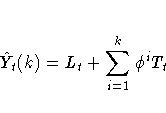
The ARIMA model equivalency to damped-trend linear exponential smoothing is the ARIMA(1,1,2) model

$(1-{\phi}B)(1-B)Y_{t} = (1-{\theta}_{1}B-{\theta}_{2}B^2) {\epsilon}_{t}$

${\theta}_{1} = 1 + {\phi} - {\alpha} - {\alpha}{\gamma}{\phi}$

${\theta}_{2} = ({\alpha} - 1){\phi}$

The moving-average form of the equation (assuming ${|{\phi}| \lt 1 }$ ) is

$Y_{t} = {\epsilon}_{t} + \sum_{j=1}^{{\infty}}{({\alpha} + {\alpha}{\gamma} {\phi}({\phi}^j - 1)/({\phi} - 1)) {\epsilon}_{t-j}}$

For damped-trend linear exponential smoothing, the additive-invertible region is

$\{ 0 \lt {\alpha} \lt 2\}$

$\{ 0 \lt {\phi}{\gamma} \lt 4/{\alpha} - 2\}$

The variance of the prediction errors is estimated as

${var}(e_{t}(k)) = {var}({\epsilon}_{t}) [ 1 + \sum_{j=1}^{k-1}{({\alpha} + {\alpha}{\gamma} {\phi}({\phi}^j - 1)/({\phi} - 1) )^2}]$

Seasonal Exponential Smoothing

The model equation for seasonal exponential smoothing is

$Y_{t} = {\mu}_{t} + s_{p}(t) + {\epsilon}_{t}$

The smoothing equations are

$L_{t} = {\alpha}(Y_{t}-S_{t-p}) + (1-{\alpha})L_{t-1}$

$S_{t} = {\delta}(Y_{t}-L_{t}) + (1-{\delta})S_{t-p}$

The error-correction form of the smoothing equations is

$L_{t} = L_{t-1} + {\alpha}e_{t}$

$S_{t} = S_{t-p} + {\delta}(1-{\alpha})e_{t}$

(Note: For missing values, e_t=0.)

The k-step prediction equation is

$\hat{Y}_{t}(k) = L_{t} + S_{t-p+k}$

The ARIMA model equivalency to seasonal exponential smoothing is the ARIMA(0,1,p+1)(0,1,0)_p model

$(1-B)(1-B^p)Y_{t} = (1 - {\theta}_{1}B - {\theta}_{2}B^p- {\theta}_{3}B^{p+1}) {\epsilon}_{t}$

${\theta}_{1} = 1 - {\alpha}$

${\theta}_{2} = 1 - {\delta}(1-{\alpha})$

${\theta}_{3} = (1 - {\alpha})({\delta} - 1)$

The moving-average form of the equation is

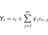
$Y_{t} = {\epsilon}_{t} + \sum_{j=1}^{{\infty}}{{\psi}_{j}{\epsilon}_{t-j}}$

${\psi}_{j} = \cases{ {\alpha} & for j\space mod p {\ne} 0\cr {\alpha}+{\delta}(1-{\alpha}) & for j\space mod p = 0\cr }$

For seasonal exponential smoothing, the additive-invertible region is

$\{ {\rm max}(-p{\alpha},0) \lt {\delta}(1-{\alpha}) \lt (2-{\alpha}) \}$

The variance of the prediction errors is estimated as

${var}(e_{t}(k)) = {var}({\epsilon}_{t}) [{\ssbeleven 1 + \sum_{j=1}^{k-1}{{\psi}_{j}^2}}]$

Winters Method -- Additive Version

The model equation for the additive version of Winters method is

$Y_{t} = {\mu}_{t} + {\beta}_{t}t + s_{p}(t) + {\epsilon}_{t}$

The smoothing equations are

$L_{t} = {\alpha}(Y_{t}-S_{t-p}) + (1-{\alpha})(L_{t-1}+T_{t-1})$

$T_{t} = {\gamma}(L_{t} - L_{t-1}) + (1-{\gamma})T_{t-1}$

$S_{t} = {\delta}(Y_{t}-L_{t}) + (1-{\delta})S_{t-p}$

The error-correction form of the smoothing equations is

$L_{t} = L_{t-1} + T_{t-1} + {\alpha}e_{t}$

$T_{t} = T_{t-1} + {\alpha}{\gamma}e_{t}$

$S_{t} = S_{t-p} + {\delta}(1-{\alpha})e_{t}$

(Note: For missing values, e_t=0.)

The k-step prediction equation is

$\hat{Y}_{t}(k) = L_{t} + kT_{t} + S_{t-p+k}$

The ARIMA model equivalency to the additive version of Winters method is the ARIMA(0,1,p+1)(0,1,0)_p model

$(1-B)(1-B^p)Y_{t} = [{\ssbeleven 1 - { \sum_{i=1}^{p+1}{{\theta}_{i}B^i}}}] {\epsilon}_{t}$

${\theta}_{j} = \cases{ 1 - {\alpha} - {\alpha}{\gamma} & j = 1 \cr -{\alpha}{\ga... ... {\delta}(1-{\alpha}) & j = p \cr (1 - {\alpha})({\delta} - 1) & j = p + 1 \cr }$

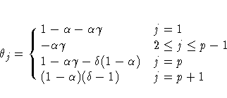
The moving-average form of the equation is

$Y_{t} = {\epsilon}_{t} + \sum_{j=1}^{{\infty}}{{\psi}_{j}{\epsilon}_{t-j}}$

${\psi}_{j} = \cases{ {\alpha}+j{\alpha}{\gamma} & for j\space mod p {\ne} 0\cr {\alpha}+j{\alpha}{\gamma}+{\delta}(1-{\alpha}),& for j\space mod p = 0\cr }$

For the additive version of Winters method (see Archibald 1990), the additive-invertible region is

$\{ {\rm max}(-p{\alpha},0) \lt {\delta}(1-{\alpha}) \lt (2-{\alpha}) \}$

$\{ 0 \lt {\alpha}{\gamma} \lt {\ssbeleven 2-{\alpha} - {\delta}(1-{\alpha})}(1-{cos}({\vartheta})\}$

where $\vartheta$ is the smallest non-negative solution to the equations listed in Archibald (1990).

The variance of the prediction errors is estimated as

${var}(e_{t}(k)) = {var}({\epsilon}_{t}) [{\ssbeleven 1 + \sum_{j=1}^{k-1}{{\psi}_{j}^2}}]$

Winters Method -- Multiplicative Version

In order to use the multiplicative version of Winters method, the time series and all predictions must be strictly positive.

The model equation for the multiplicative version of Winters method is

$Y_{t} = ({\mu}_{t} + {\beta}_{t}t) s_{p}(t) + {\epsilon}_{t}$

The smoothing equations are

$L_{t} = {\alpha}(Y_{t}/S_{t-p}) + (1-{\alpha})(L_{t-1}+T_{t-1})$

$T_{t} = {\gamma}(L_{t} - L_{t-1}) + (1-{\gamma})T_{t-1}$

$S_{t} = {\delta}(Y_{t}/L_{t}) + (1-{\delta})S_{t-p}$

The error-correction form of the smoothing equations is

$L_{t} = L_{t-1} + T_{t-1} + {\alpha}e_{t}/S_{t-p}$

$T_{t} = T_{t-1} + {\alpha}{\gamma}e_{t}/S_{t-p}$

$S_{t} = S_{t-p} + {\delta}(1-{\alpha})e_{t}/L_{t}$

(Note: For missing values, e_t=0.)

The k-step prediction equation is

$\hat{Y}_{t}(k) = (L_{t} + kT_{t})S_{t-p+k}$

The multiplicative version of Winters method does not have an ARIMA equivalent; however, when the seasonal variation is small, the ARIMA additive-invertible region of the additive version of Winters method described in the preceding section can approximate the stability region of the multiplicative version.

The variance of the prediction errors is estimated as

${var}(e_{t}(k)) = {var}({\epsilon}_{t}) [{\ssbeleven \sum_{i=0}^{{\infty}}{\sum_{j=0}^{p-1}{({\psi}_{j+ip}S_{t+k}/S_{t+k-j})^2 }}}]$

where ${{\psi}_{j}}$ are as described for the additive version of Winters method, and ${{\psi}_{j} = 0}$ for ${j \ge k}$ .

Chapter Contents
Previous
Next
Top