Chapter Contents
Previous
Next
|
Chapter Contents |
Previous |
Next |
| SAS Macros and Functions |
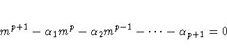
Consider the (p+1)th order autoregressive time series

and its characteristic equation
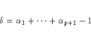
If all the characteristic roots are less than 1 in absolute value, Yt is stationary. Yt is nonstationary if there is a unit root. If there is a unit root, the sum of the autoregressive parameters is 1, and, hence, you can test for a unit root by testing whether the sum of the autoregressive parameters is 1 or not. For convenience, the model is parameterized as
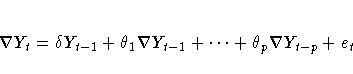
where ![]() and
and

The estimators are obtained by regressing
![]() on
on
![]() .The t statistic of the ordinary least squares estimator
of
.The t statistic of the ordinary least squares estimator
of ![]() is the test statistic for the unit root test.
is the test statistic for the unit root test.
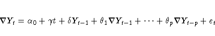
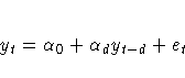
If the TREND=1 option is used, the autoregressive model includes
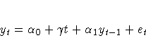
a mean term ![]() .If TREND=2, the model also includes a time trend term and the
model is as follows:
.If TREND=2, the model also includes a time trend term and the
model is as follows:
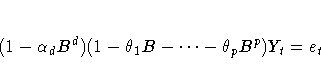
For testing for a seasonal unit root, consider the multiplicative model
Let ![]() .The test statistic is calculated in the following steps:
.The test statistic is calculated in the following steps:
The t ratio for the estimate of ![]() produced by the second step
is used as a test statistic for testing for a seasonal unit root.
The estimates of
produced by the second step
is used as a test statistic for testing for a seasonal unit root.
The estimates of
![]() are obtained by adding the estimates of
are obtained by adding the estimates of
![]() from the second step to
from the second step to
![]() from the first step.
The estimates of
from the first step.
The estimates of ![]() and
and ![]() are saved in the OUTSTAT= data set if the OUTSTAT= option is specified.
are saved in the OUTSTAT= data set if the OUTSTAT= option is specified.
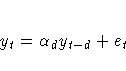
The series (1-Bd)Yt is assumed to be stationary, where d is the value of the DLAG= option.
If the OUTSTAT= option is specified,
the OUTSTAT= data set contains estimates
![]() .
.
If the series is an ARMA process, a large value of the AR= option may be desirable in order to obtain a reliable test statistic. To determine an appropriate value for the AR= option for an ARMA process, refer to Said and Dickey (1984).
There are several different versions of the Dickey-Fuller test. The PROBDF function supports six versions, as selected by the type argument. Specify the type value that corresponds to the way that you calculated the test statistic x.
The last two characters of the type value specify the kind of regression model used to compute the Dickey-Fuller test statistic. The meaning of the last two characters of the type value are as follows.


Refer to Dickey and Fuller (1979) and Dickey, Hasza, and Fuller (1984) for more information about the Dickey-Fuller test null distribution. The preceding formulas are for the basic Dickey-Fuller test. The PROBDF function can also be used for the augmented Dickey-Fuller test, in which the error term et is modeled as an autoregressive process; however, the test statistic is computed somewhat differently for the augmented Dickey-Fuller test. Refer to Dickey, Hasza, and Fuller (1984) and Hamilton (1994) for information about seasonal and nonseasonal augmented Dickey-Fuller tests.
The PROBDF function is calculated from approximating functions fit to empirical quantiles produced by Monte Carlo simulation employing 108 replications for each simulation. Separate simulations were performed for selected values of n and for d=1,2,4,6,12.
The maximum error of the PROBDF function is approximately
![]() for d in the set (1,2,4,6,12)
and may be slightly larger for other d values.
(Because the number of simulation replications used to produce
the PROBDF function is much greater than the 60,000 replications used by
Dickey and Fuller (1979) and Dickey, Hasza, and Fuller (1984),
the PROBDF function can be expected to produce results that are
substantially more accurate than the critical values reported in
those papers.)
for d in the set (1,2,4,6,12)
and may be slightly larger for other d values.
(Because the number of simulation replications used to produce
the PROBDF function is much greater than the 60,000 replications used by
Dickey and Fuller (1979) and Dickey, Hasza, and Fuller (1984),
the PROBDF function can be expected to produce results that are
substantially more accurate than the critical values reported in
those papers.)
|
Chapter Contents |
Previous |
Next |
Top |
Copyright © 1999 by SAS Institute Inc., Cary, NC, USA. All rights reserved.