Chapter Contents
Previous
Next
|
Chapter Contents |
Previous |
Next |
| The AUTOREG Procedure |
Consider the series yt, which follows the GARCH process. The conditional distribution of the series Y for time t is written

where ![]() denotes all available information at time
t-1.
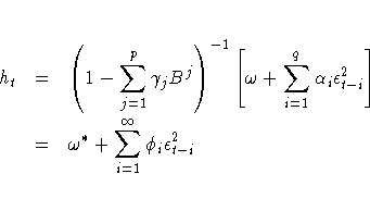
The conditional variance ht is
denotes all available information at time
t-1.
The conditional variance ht is

where


The GARCH(p,q) model reduces to the ARCH(q) process when p=0. At least one of the ARCH parameters must be nonzero (q > 0). The GARCH regression model can be written


where ![]() .
.
In addition, you can consider the model with disturbances following an autoregressive process and with the GARCH errors. The AR(m)-GARCH(p,q) regression model is denoted


where B is a backshift operator.
Therefore, ![]() if
if
![]() and
and
![]() .
Assume that the roots of
the following polynomial equation are inside the unit circle:
.
Assume that the roots of
the following polynomial equation are inside the unit circle:

Define n=max(p,q).
The coefficient ![]() is written
is written

Nelson and Cao (1992) proposed the finite inequality constraints for GARCH(1,q) and GARCH(2,q) cases. However, it is not straightforward to derive the finite inequality constraints for the general GARCH(p,q) model.
For the GARCH(1,q) model, the nonlinear inequality constraints are

For the GARCH(2,q) model, the nonlinear inequality constraints are

where ![]() and
and ![]() are the roots of
are the roots of
![]() .
.
For the GARCH(p,q) model with p > 2, only max(q-1,p)+1 nonlinear
inequality constraints (![]() for k=0 to max(q-1,p))
are imposed, together with the in-sample positivity
constraints of the conditional variance ht.
for k=0 to max(q-1,p))
are imposed, together with the in-sample positivity
constraints of the conditional variance ht.
the GARCH process is weakly stationary since the mean, variance, and autocovariance are finite and constant over time. However, this condition is not sufficient for weak stationarity in the presence of autocorrelation. For example, the stationarity condition for an AR(1)-GARCH(p,q) process is

When the GARCH process is stationary,
the unconditional variance of ![]() is computed as
is computed as

GARCH(p,q) conditional variance.
Sometimes, the multistep forecasts of the variance do not approach the
unconditional variance when the model is integrated in variance; that is,
![]() .
.
The unconditional variance for the IGARCH model does not exist. However, it is interesting that the IGARCH model can be strongly stationary even though it is not weakly stationary. Refer to Nelson (1990) for details.

where
![g( z_{t}) = {\theta} z_{t}+{\gamma}[{| z_{t}|}
-E{| z_{t}|}]](images/auteq124.gif)

The coefficient of the second term in g( zt) is set to be
1 (![]() =1) in our formulation. Note that
=1) in our formulation. Note that
![]() if
if
![]() .
The properties of the EGARCH model are summarized as follows:
.
The properties of the EGARCH model are summarized as follows:

When et is assumed to have a standard normal distribution
(![]() ), the likelihood function is
given by
), the likelihood function is
given by
![l = \sum_{t=1}^N{\frac{1}2[-{\ln}(2{\pi})
-{\ln}( h_{t})-
{{\epsilon}_{t}^2 \over h_{t}}]}](images/auteq139.gif)
where ![]() and
ht is the conditional variance.
When the GARCH(p,q)-M model is estimated,
and
ht is the conditional variance.
When the GARCH(p,q)-M model is estimated,
![]() .
When there are no regressors, the residuals
.
When there are no regressors, the residuals
![]() are denoted as yt or
are denoted as yt or
![]() .
.
If et has the standardized Student's t distribution the log likelihood function for the conditional t distribution is

where ![]() is the gamma function and
is the gamma function and ![]() is the degree of freedom (
is the degree of freedom (![]() ).
Under the conditional t distribution, the additional parameter
).
Under the conditional t distribution, the additional parameter
![]() is estimated. The log likelihood function for
the conditional t distribution converges to the log likelihood
function of the conditional normal GARCH model as
is estimated. The log likelihood function for
the conditional t distribution converges to the log likelihood
function of the conditional normal GARCH model as
![]() .
.
The likelihood function is maximized via either the dual quasi-Newton
or trust region algorithm. The default is the dual quasi-Newton algorithm.
The starting values for the regression parameters ![]() are
obtained from the OLS estimates.
When there are autoregressive parameters
in the model, the initial values are obtained from the Yule-Walker estimates.
The starting value 1.0-6 is used for the GARCH process parameters.
are
obtained from the OLS estimates.
When there are autoregressive parameters
in the model, the initial values are obtained from the Yule-Walker estimates.
The starting value 1.0-6 is used for the GARCH process parameters.
The variance-covariance matrix is computed using the Hessian matrix.
The dual quasi-Newton method approximates the Hessian matrix while the
quasi-Newton method gets an approximation of the inverse of Hessian.
The trust region method uses the Hessian matrix obtained using numerical
differentiation.
When there are active constraints, that is, ![]() ,
the variance-covariance matrix is given by
,
the variance-covariance matrix is given by
![V(\hat{{\theta}}) =
H^{-1}[I - Q' (Q
H^{-1}Q')^{-1}Q H^{-1}]](images/auteq150.gif)
where
![]() and
and ![]() .
Therefore, the variance-covariance matrix without active
constraints reduces to
.
Therefore, the variance-covariance matrix without active
constraints reduces to ![]() .
.
|
Chapter Contents |
Previous |
Next |
Top |
Copyright © 1999 by SAS Institute Inc., Cary, NC, USA. All rights reserved.