| Nonlinear Optimization Examples |
Finite Difference Approximations of Derivatives
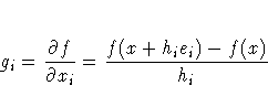
If the optimization technique needs first- or second-order
derivatives and you do not specify the corresponding
IML modules "grd", "hes", "jac", or
"jacnlc", the derivatives are approximated by finite
difference formulas using only calls of the module "fun".
If the optimization technique needs second-order derivatives and
you specify the "grd" module but not the "hes" module,
the subroutine approximates the second-order derivatives by finite
differences using n or 2n calls of the "grd" module.
The eighth element of the opt argument specifies
the type of finite difference approximation used to
compute first- or second-order derivatives and whether
the finite difference intervals, h, should be computed
by an algorithm of Gill, Murray, Saunders, and Wright (1983).
The value of opt[8] is a two-digit integer, ij.
- If opt[8] is missing or j=0, the fast
but not very precise forward difference formulas
are used; if
 , the numerically more
expensive central difference formulas are used.
, the numerically more
expensive central difference formulas are used.
- If opt[8] is missing or
 ,
the finite difference intervals h are based only on the
information of par[8] or par[9], which specifies
the number of accurate digits to use in evaluating the
objective function and nonlinear constraints, respectively.
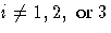
If i = 1,2, or3, the intervals are computed with
an algorithm by Gill, Murray, Saunders, and Wright (1983).
For i=1, the interval is based on the behavior of the
objective function; for i=2, the interval is based on the
behavior of the nonlinear constraint functions; and for
i=3, the interval is based on the behavior of both the
objective function and the nonlinear constraint functions.
,
the finite difference intervals h are based only on the
information of par[8] or par[9], which specifies
the number of accurate digits to use in evaluating the
objective function and nonlinear constraints, respectively.
If i = 1,2, or3, the intervals are computed with
an algorithm by Gill, Murray, Saunders, and Wright (1983).
For i=1, the interval is based on the behavior of the
objective function; for i=2, the interval is based on the
behavior of the nonlinear constraint functions; and for
i=3, the interval is based on the behavior of both the
objective function and the nonlinear constraint functions.
Forward Difference Approximations
- First-order derivatives: n additional function
calls are needed.
- Second-order derivatives based on function calls
only, when the "grd" module is not specified
(Dennis and Schnabel 1983): for a dense Hessian
matrix, n+n2/2 additional function calls are needed.

- Second-order derivatives based on gradient calls, when
the "grd" module is specified (Dennis and Schnabel
1983): n additional gradient calls are needed.

Central Difference Approximations
- First-order derivatives: 2n
additional function calls are needed.

- Second-order derivatives based on function calls
only, when the "grd" module is not specified
(Abramowitz and Stegun 1972): for a dense Hessian
matrix, 2n+2n2 additional function calls are needed.
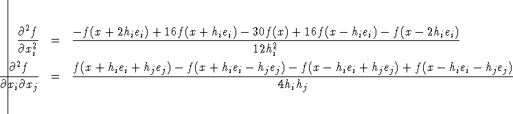
- Second-order derivatives based on gradient
calls, when the "grd" module is specified:
2n additional gradient calls are needed.

The step sizes hj, j = 1, ... ,n, are defined as follows:
- For the forward-difference approximation of
first-order derivatives using only function calls and
for second-order derivatives using only gradient calls,
![h_j = \sqrt[2]{\eta_j} (1 + | x_j|)](images/i11eq27.gif) .
. - For the forward-difference approximation of
second-order derivatives using only function
calls and for central-difference formulas,
![h_j = \sqrt[3]{\eta_j} (1 + | x_j|)](images/i11eq28.gif) .
.
If the algorithm of Gill, Murray, Saunders, and Wright
(1983) is not used to compute  , a constant value
 is used depending on the value of par[8].
- If the number of accurate digits is specified by
par[8]=k1, then
 is set to 10-k1.
- If par[8] is not specified, is
set to the machine precision,
 .
.
If central difference formulas are not specified, the
optimization algorithm will switch automatically from
the forward-difference formula to a corresponding
central-difference formula during the iteration process
if one of the following two criteria is satisfied:
- The absolute maximum gradient element is less
than or equal to 100 times the ABSGTOL threshold.
- The term on the left of the GTOL criterion
is less than or equal to
max(1E-6, 100×GTOL threshold).
The 1E-6 ensures that the switch is performed
even if you set the GTOL threshold to zero.
The algorithm of Gill, Murray, Saunders, and Wright (1983)
that computes the finite difference intervals hj can
be very expensive in the number of function calls it uses.
If this algorithm is required, it is performed
twice, once before the optimization process
starts and once after the optimization terminates.
Many applications need considerably more
time for computing second-order derivatives
than for computing first-order derivatives.
In such cases, you should use a quasi-Newton
or conjugate gradient technique.
If you specify a vector, c, of nc nonlinear constraints
with the "nlc" module but you do not specify the
"jacnlc" module, the first-order formulas can be
used to compute finite difference approximations of the
nc ×n Jacobian matrix of the nonlinear constraints.

You can specify the number of accurate digits
in the constraint evaluations with par[9].
This specification also defines the
step sizes hj, j = 1, ... ,n.
Note: If you are not able to specify analytic
derivatives and if the finite-difference approximations
provided by the subroutines are not good enough to solve
your optimization problem, you may be able to implement
better finite-difference approximations with the "grd",
"hes", "jac", and "
jacnlc" module arguments.
Copyright © 1999 by SAS Institute Inc., Cary, NC, USA. All rights reserved.