Robust Regression Examples

Overview

SAS/IML has three subroutines that can be used for outlier detection and robust regression. The Least Median of Squares (LMS) and Least Trimmed Squares (LTS) subroutines perform robust regression (sometimes called resistant regression). These subroutines are able to detect outliers and perform a least-squares regression on the remaining observations. The Minimum Volume Ellipsoid Estimation (MVE) subroutine can be used to find the minimum volume ellipsoid estimator, which is the location and robust covariance matrix that can be used for constructing confidence regions and for detecting multivariate outliers and leverage points. Moreover, the MVE subroutine provides a table of robust distances and classical Mahalanobis distances. The LMS, LTS, and MVE subroutines and some other robust estimation theories and methods were developed by Rousseeuw (1984) and Rousseeuw and Leroy (1987). Some statistical applications for MVE are described in Rousseeuw and Van Zomeren (1990).

Whereas robust regression methods like L1 or Huber M-estimators reduce the influence of outliers only (compared to least-squares or L2 regression), resistant regression methods like LMS and LTS can completely disregard influential outliers (sometimes called leverage points) from the fit of the model. The algorithms used in the LMS and LTS subroutines are based on the PROGRESS program by Rousseeuw and Leroy (1987). Rousseeuw and Hubert (1996) prepared a new version of PROGRESS to facilitate its inclusion in SAS software, and they have incorporated several recent developments. Among other things, the new version of PROGRESS now yields the exact LMS for simple regression, and the program uses a new definition of the robust coefficient of determination (R²). Therefore, the outputs may differ slightly from those given in Rousseeuw and Leroy (1987) or those obtained from software based on the older version of PROGRESS. The MVE algorithm is based on the algorithm used in the MINVOL program by Rousseeuw (1984).

The three SAS/IML subroutines are designed for

LMS: minimizing the hth ordered squared residual
LTS: minimizing the sum of the h smallest squared residuals
MVE: minimizing the volume of an ellipsoid containing h points

where h is defined in the range

$\frac{N}2 + 1 \leq h \leq \frac{3N}4 + \frac{n+1}4$

In the preceding equation, N is the number of observations and n is the number of regressors. ^* The value of h determines the breakdown point, which is "the smallest fraction of contamination that can cause the estimator T to take on values arbitrarily far from T(Z)" (Rousseeuw and Leroy 1987, p.10). Here, T denotes an estimator and T(Z) applies T to a sample Z.

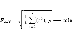
For each parameter vector b = (b₁, ... ,b_n), the residual of observation i is r_i = y_i - x_i b. You then denote the ordered, squared residuals as

$(r^2)_{1:N} \leq ... \leq (r^2)_{N:N}$

The objective functions for the LMS and LTS optimization problems are defined as follows:

LMS
$F_{\rm LMS} = (r^2)_{h:N} \longrightarrow \min$
Note that, for h= N/2+1, the hth quantile is the median of the squared residuals. The default h in PROGRESS is h = [ [(N+n+1)/2] ], which yields the breakdown value (where [k] denotes the integer part of k).
LTS
$F_{\rm LTS} = \sqrt{ \frac{1}h \sum_{i=1}^h (r^2)_{i:N} } \longrightarrow \min$
MVE
The objective function for the MVE optimization problem is based on the hth quantile d_h:N of the Mahalanobis-type distances d = (d₁, ... ,d_N),
$F_{\rm MVE} = \sqrt{d_{h:N} {det}(C)} \longrightarrow \min$
subject to $d_{h:N} = \sqrt{\chi^2_{n,0.5}}$ , where C is the scatter matrix estimate, and the Mahalanobis-type distances are computed as
$d = {diag}(\sqrt{ (X - T)^T C^{-1} (X - T)} )$
where T is the location estimate.

Because of the nonsmooth form of these objective functions, the estimates cannot be obtained with traditional optimization algorithms. For LMS and LTS, the algorithm, as in the PROGRESS program, selects a number of subsets of n observations out of the N given observations, evaluates the objective function, and saves the subset with the lowest objective function. As long as the problem size enables you to evaluate all such subsets, the result is a global optimum. If computer time does not permit you to evaluate all the different subsets, a random collection of subsets is evaluated. In such a case, you may not obtain the global optimum.

Note that the LMS, LTS, and MVE subroutines are executed only when the number N of observations is over twice the number n of explanatory variables x_j (including the intercept), that is, if N > 2n.

Flow Chart for LMS, LTS, and MVE

Chapter Contents
Previous
Next
Top